Energy-selective quantum search with Ising Hamiltonian phase oracles

A. S. Plyashechnik, A. A. Zhukov, A. V. Lebedev, W. V. Pogosov · arXiv:2606.03380 · new submission, announced 2026-06-03 · score 9/10 (HIGH)

Abstract

Ising Hamiltonians are basic models of disordered magnets and a standard language for quantum and classical optimization. We study an energy-selective quantum search primitive in which the physical evolution exp(-iTH) is used directly as a Hamiltonian phase oracle. Unlike a Boolean oracle, this oracle marks configurations continuously by their phases and selects a finite resonance band rather than a preassigned marked set. We show that alternating it with the Grover diffusion operator nevertheless produces a Grover-type amplification peak. An exact spectral recurrence and a generating-function representation determine the peak position, width, and height. For an annealed Gaussian density of states, target energies in a high-density tail require Θ(√(2ⁿ/M)) oracle calls when the resonance contains M configurations. For random Ising spectra, overlap-induced correlations shift and distort the peak; spectral symmetrization and iterative calibration remove this detuning for prescribed-energy targeting.

Executive summary

The authors replace Grover's Boolean phase oracle with the continuous-phase operator U_T = exp(-iTH) of an Ising Hamiltonian itself, then prove that alternating U_T with the standard Grover diffuser still yields a quadratic-speedup amplification peak — at a target energy E* = π/T selected by the operator's free parameter T. The selected subspace is generated self-consistently by the local spectral density (not specified externally as in Boolean Grover), and reaches it in Θ(√(2ⁿ/M)) oracle calls, with each call costing only the O(n²) commuting ZZ rotations needed to Trotter-implement exp(-iTH) exactly. For Yuan this is directly load-bearing: it is the closest possible methodological neighbour to Y4 (Grover × cardinality-structured search), and the √(2ⁿ/M) scaling matches Y4's √(C(n,k)/M) when the energy resonance band plays the role of the cardinality-feasible subspace.

Main contribution

The paper develops a complete spectral theory of an "Ising Grover" iterate W_T = D_ξ U_T with D_ξ = 2|ξ⟩⟨ξ| - I the diffuser about the uniform state. The amplitudes a_K(E) satisfy an exact one-dimensional recurrence (Eq. 11) in energy, whose generating-function solution (Eq. 19) factorises into a resonance kernel and a spectral susceptibility C_r(φ) = 2G(-re^{iφ}) - 1, where G is the generating function of the characteristic-function samples g_m = 2^-n Tr exp(-imTH) — the partition function at imaginary inverse temperature β = imT. The local zero of Im C_r determines the resonance position; its slope and real part determine width and saturation height. For the annealed Gaussian density of states this gives K_peak ~ n^μ-3/2 2^n/2 and resonance cardinality M_peak ~ n^3-2μ, recovering Grover scaling. For correlated random-Ising spectra (overlap-correlated levels rather than independent random energies), spin-glass correlations shift the resonance by φ_0 = O(n^-3) rms and can also depress the peak height — both effects are fixed analytically and corrected via either (i) ancilla-based spectral symmetrization or (ii) an iteratively self-calibrating evolution time.

Key theorems / lemmas / algorithms

Algorithm (Sec. II.A): Iterate W_T = D_ξ U_T with U_T = ∏_i exp(-iTh_iZ_i) ∏_i<j exp(-2iTJ_ijZ_iZ_j) — exact, no Trotter error, since all Ising terms commute.
Spectral recurrence (Eq. 11): a_K(E) = 2∫ e^-iTE' a_{K-1}(E') f(E') dE' − e^-iTE a_{K-1}(E). Reduces the full 2ⁿ-dim dynamics to a 1D scalar problem in energy.
Generating-function solution (Eq. 19): Closed-form integral representation of a_{K-1}(E) involving the spectral response C_r(φ) = 2G(-re^{iφ}) - 1.
Annealed Gaussian theorem (Sec. IV): K_peak ~ √(2ⁿ/M_peak) with M_peak ~ n^3-2μ, recovering Grover scaling for a self-generated marked band.
Correlation displacement (Eq. 33, Eq. 34): φ_0 = O(n^-3) rms; energy displacement δE_shift = O(n^{-1/2 - 1}})}. Derived from the exact covariance E[g_m g_ℓ*] in Eq. 27 evaluated over Hamming-distance shells.
Peak-height bound (Eq. 39): A_max^(Ising) ≤ min[2^n/2, n^μ-3/22^n/2, 2^(1-d*)n/2n^...], with the third term a genuinely correlation-induced reduction (d* ≈ 0.0194, s* ≈ 0.308) below the annealed prediction.
Spectral symmetrization (Eq. 41): H̃ = Z_a ⊗ H doubles the spectrum to ±E_j, making g̃_m real and forcing φ_0 = 0; cost is three-body terms Z_aZ_iZ_j.
Iterative time calibration (Eqs. 47–49): Self-consistent map T ← (π + φ_0(T))/E* converges in O(n/ln n) updates with contraction factor O(n^-3).

Detailed walkthrough

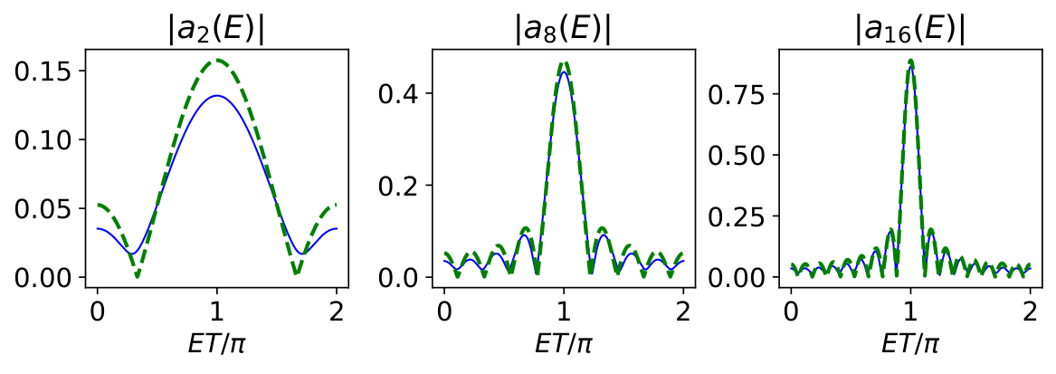
Section II frames the setup. The Ising Hamiltonian H = ∑_i h_iZ_i + 2∑_i<j J_ijZ_iZ_j is diagonal in the computational basis, so U_T = exp(-iTH) assigns a configuration-dependent phase exp(-iTE_s) — a continuous spectral oracle rather than a Boolean one. The key conceptual move is to ask whether alternating this with the Grover diffuser D_ξ still produces coherent amplification when no sharply marked subspace exists. The answer is yes, under a condition: a configuration becomes resonant when TE_s ≈ π (mod 2π), and the diffusion step couples energies only through their spectral average, so a finite phase neighbourhood around TE = π is amplified collectively.

Section III is the analytic heart. Equation 11 is the recurrence for energy-resolved amplitudes; Eq. 19 expresses a_{K-1}(E) as a contour integral of a "resonance kernel" divided by C_r(φ) = 2G(-re^{iφ}) - 1 where G(z) = ∑ g_m z^m. The radius r is an auxiliary parameter (the authors later fix 1-r = O(1/K)). The local linearisation C_r(φ) ≈ ε_eff + iκ_C(φ - φ_0) immediately gives the peak position (where Im C_r vanishes), the phase width ε_eff/|κ_C|, and the saturation height |κ_C|/ε_eff. This is a clean, very general susceptibility framework: any spectrum that gives g_m compatible with a singular response near φ = 0 yields Grover-type behaviour.

Section IV instantiates the framework for the annealed Gaussian density f_G(E) with variance Σ_n² = 2n(n-1)σ_J² + nσ_h². The characteristic-function samples are g_m = exp[-(mΣ_nT)²/2]; with the natural dimensionless tail parameter a = (Σ_nT)²/2 << 1 one obtains ε_G = 2√(π/a) exp(-π²/(4a)). The "high-density tail" regime is defined by parametrising the local mean spacing as Δ_n ~ n^μ 2^-n/2, which forces the target energy E* = O(n^3/2). The arithmetic collapses to K_peak ~ √(2ⁿ/M_peak) with M_peak ~ n^3-2μ — Grover scaling for a target band whose cardinality is determined by spectral physics rather than by user choice. For μ = 3/2 one selects O(1) levels; for smaller μ the resonance band grows polynomially.

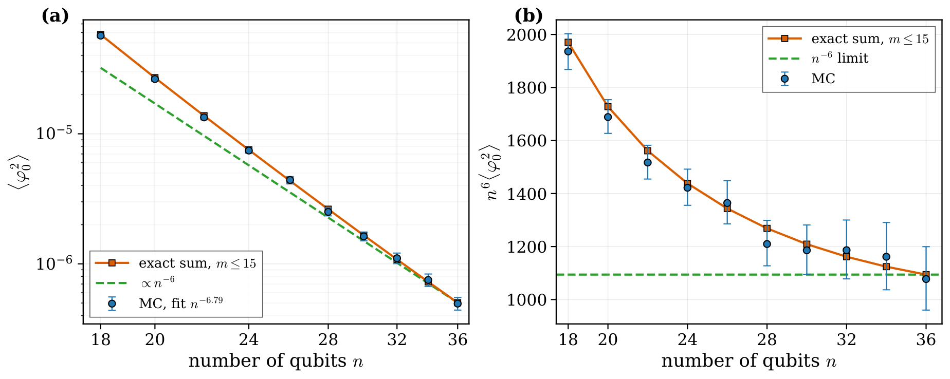
Section V is where the spin-glass physics becomes load-bearing. The independent-energy approximation (random-energy model) gets the average density right but misses overlap-induced level correlations. Equation 27 gives the exact two-point covariance E[g_m g_ℓ*] = 2^-n exp{-αn[(n-1)(m²+ℓ²) + 2mℓ]} ∑_q C(n,q) exp[2αmℓ(n-2q)²] with q the Hamming distance between configurations. The q = 0, n terms give a persistent O(2^-n/2) noise floor in the g_m sequence that propagates into C_r near the unit circle. The upshot (Eq. 32-34) is that the resonance centre φ_0 is displaced by an O(n^-3) rms phase — small on spectral scales but large compared with the exponentially narrow resonance width.

Section VI addresses prescribed-energy targeting. The symmetrization trick (Eq. 41-42) adds an ancilla and replaces H by Z_a ⊗ H, doubling the spectrum to ±E_j and making g̃_m manifestly real — hence φ_0 = 0 exactly. The cost is three-body Z_aZ_iZ_j terms. Alternatively the time calibration T ← (π + φ_0(T))/E* is shown (Eq. 47-49) to converge in O(n/ln n) updates using only the measured bit string and its classical Ising energy — natural for an experimental loop. Section VII assembles total cost: each oracle call is O(n²) commuting ZZ rotations, so the gate cost of producing a resonance state is O(n² √(2ⁿ/M_peak)).

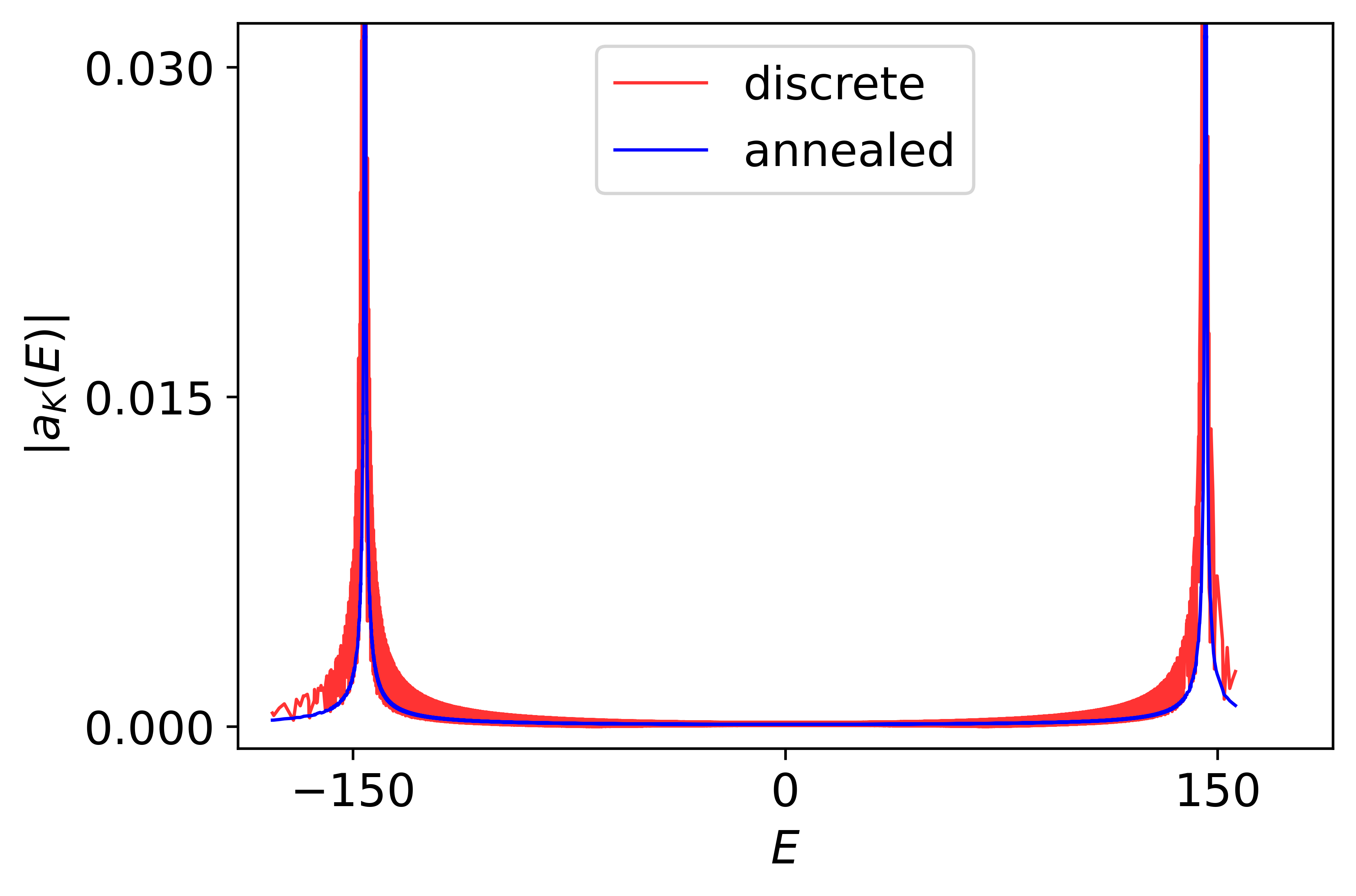
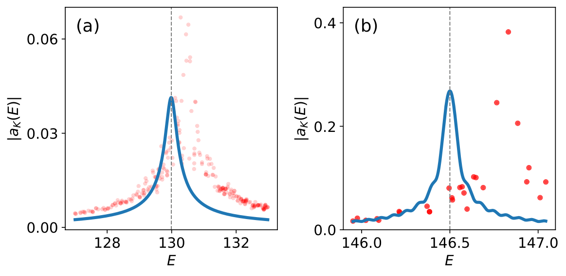
Section VIII shows numerics for n = 24. Figure 1 verifies the Gaussian local-response approximation. Figure 2 compares the discrete random Ising response with the annealed Gaussian: both show resonances near ET = ±π, but the Ising peak is shifted and distorted. Figure 3 zooms in on the resonance for two target energies, showing the predicted scaling of width and height with μ. The n = 18,...,36 scan in Fig. 4 verifies √⟨φ_0²⟩ = O(n^-3).

Figures

Figure 1. Amplification profile for an annealed Gaussian spectrum near the principal phase resonance ET = π. Horizontal axis is dimensionless phase ET/π; panels show amplitude magnitude after K = 2, 8, 16 iterations. Solid: exact spectral recurrence. Dashed: local resonant approximation. Parameters give ΣT ≈ 0.72. Agreement near ET/π = 1 illustrates that the local response captures the growth and narrowing of the Gaussian resonance.

Ising vs Gaussian energy-space amplification — Figure 2. Energy-space amplification profile for a single zero-field random Ising instance (n = 24, h_i = 0, J_ij ~ N(0,1)) compared with the annealed Gaussian prediction. Red: discrete Ising spectrum. Blue: annealed Gaussian. Both develop resonances near ET = ±π, but the discrete Ising response is shifted and distorted by spectral correlations.

Zoom of positive-energy resonance — Figure 3. Zoom of the positive-energy resonance at n = 24. Blue: annealed Gaussian. Red points: amplitudes on the discrete Ising energy levels. Dashed line: Gaussian target energy E* = π/T. Panel (a): denser tail (μ ≈ 0.6), broader/lower peak. Panel (b): sparser tail (μ ≈ 1.2), sharper/higher peak. In both, the discrete Ising peak is displaced from the Gaussian target — the realization-dependent shift φ_0.

phi0 scaling with system size — Figure 4. Scaling of the correlation-induced resonance displacement in the zero-field random Ising ensemble. σ_J = 1, J_ij ~ N(0,1), h_i = 0, μ = 3/2, truncated characteristic function with m ≤ 15. (a) Disorder-averaged ⟨φ_0²⟩ for n = 18,...,36; circles are Monte Carlo, squares are the finite-n covariance sum, dashed line is the asymptotic n^-6 law. (b) Scaled quantity n⁶⟨φ_0²⟩ showing finite-size drift toward the asymptotic plateau. RMS displacement obeys √⟨φ_0²⟩ = O(n^-3).

Citations to Yuan's papers

No direct citation to any of Y1–Y6 found in bibliography.

Overlap with Y1–Y6

Y4 (Grover + ADMM for cardinality-constrained binary optimization) — strongest overlap. Both papers establish O(√(D/M)) Grover-type scaling for structured feasible spaces — Y4 with D = C(n,k) (fixed cardinality), this paper with D = 2ⁿ and M = M_peak the resonance-band cardinality determined by the local Ising density of states. The mechanisms differ at the oracle level: Y4 constructs an explicit superposition over C(n,k) feasible states and rotates inside it; this paper uses the problem Hamiltonian as a continuous spectral oracle and generates the marked band dynamically. The "effective marked set generated by the oracle's own physics" idea here is conceptually adjacent to Y4's hard-mixer / feasibility-preserving philosophy.
Y1 (iterative warm-started QAOA) — method-side resonance: both papers iterate a parametrised unitary (W_T here, U_QAOA(β,γ) in Y1) and use measurement feedback to update a single scalar parameter (T here, the warm-start angle in Y1) toward convergence. The contraction argument in Sec. VI.B of this paper has the same "polynomial-overhead feedback loop" character as Y1's iterative refinement.
Y3 (QAOA DGMVP portfolio) — adjacent: this paper analyses an Ising/QUBO-encoded optimisation problem and discusses spectral structure of the cost landscape; Y3 analyses QAOA on Ising-encoded portfolio problems and finds that noise destroys advantage but shot-noise scaling is favourable. Both treat the spectral / landscape structure of disordered Ising-type cost Hamiltonians, but with different algorithms.
Y2 (quasi-binary QAOA) — peripheral: shared scope of constrained Ising-encoded combinatorial optimisation, but Y2's mixer-design approach has no counterpart here.
Y5 (GW SDP via Gibbs states) — peripheral: this paper's "g_m = 2^-n Tr exp(-imTH) as imaginary-temperature partition function" framing is conceptually adjacent to Y5's use of quantum Gibbs states as primitives, but the algorithmic target is unrelated.
Y6 (PBR test) — none.

Recommended action for Yuan

Cite in the next Y4-line paper. The scaling Θ(√(2ⁿ/M)) for a self-generated marked band is the closest published cousin to Y4's O(√(C(n,k)/M)). The two results sit cleanly side-by-side and frame the Grover landscape: Y4 imposes structure on the feasible set; this paper extracts structure from the cost Hamiltonian's spectrum.
Read deeper. Sec. III's generating-function machinery (the susceptibility C_r(φ) and its local linearisation) is a clean, transportable formalism. It may give a Y4-style quadratic-speedup bound for cardinality-constrained optimisation when the cost has structured spectral correlations (e.g. portfolio covariance with low-rank corrections). Worth at least a back-of-envelope check.
Compare on an Ising portfolio instance. The DGMVP cost Hamiltonian (Y3) is exactly an Ising-with-fields encoding. Running the energy-selective resonance against a known QAOA baseline on a small DGMVP instance would be a one-day numerical experiment that directly tests whether the resonance primitive recovers the Y3 portfolio ground state competitively.