Benchmarking Quantum Annealing for a Greenhouse-Inspired Control QUBO

Hamzeh Alavirad, Maryam Bahrami Zanjani (QUSMOS) · arXiv:2605.27670 · submitted 2026-05-28 · score 8/10

Abstract

We benchmark current annealing-based optimization workflows on a greenhouse-inspired quadratic unconstrained binary optimization problem for binary heater scheduling, where the horizon H denotes the number of hourly control decisions. For the main one-day instance (H=24), all solver outputs are decoded back into heater schedules and evaluated in the original greenhouse simulator using the same physical objective and feasibility criterion. Classical simulated annealing and path-integral simulated quantum annealing produce feasible near-optimal solutions in all repetitions, with best objectives close to the exact optimum. In contrast, the tested D-Wave Leap Hybrid BQM workflow is less reliable and does not outperform the classical baselines under 15–60 s requested time limits. Direct D-Wave QPU execution on reduced instances remains feasible in all runs and recovers the exact optimum for H=10 and H=12, but the exact-hit rate drops from 5/10 to 2/10 and then to 0/10 at H=14, with substantially higher variance than the classical baselines. The results do not indicate quantum advantage, but provide a reproducible, physically decoded benchmark that exposes the current strengths and limitations of classical, hybrid, and direct quantum annealing workflows on structured control QUBOs.

Executive summary

This is exactly the kind of negative-result QUBO benchmark Yuan’s Y3 paper builds its case on: a structured combinatorial control problem (binary heater scheduling over a 24-hour horizon) is mapped to a 312-variable BQM, solved on D-Wave hardware (Advantage2_system1) and Leap Hybrid BQM, and compared against an exact ground truth and against classical simulated annealing (SA) and path-integral simulated quantum annealing (PIA). Across every comparison the classical baselines win on mean decoded objective, and the QPU’s exact-hit rate degrades from 5/10 at H=10 to 0/10 at H=14. The paper makes no quantum-advantage claim and explicitly contextualises its findings as a reproducible, physically-decoded benchmark. For Yuan, the relevance is direct: it is independent confirmation that, on a structured constrained-binary-optimisation QUBO at the scales currently reachable on real hardware, simulated annealing remains a strong baseline that hybrid/QPU workflows fail to beat — the same headline conclusion as Y3’s thermal-regime DGMVP portfolio result.

Main contribution

The contribution is twofold. (1) A reproducible greenhouse-inspired control QUBO benchmark with a two-state thermal model, exogenous solar/outdoor-temperature/electricity-price forcing, a quadratic growth proxy, hard temperature-bound constraints encoded via binary slack variables, and a switching-penalty term. The H=24 instance yields a 312-variable BQM with 4 596 quadratic couplers (24 control bits + 288 slack bits with M=6 slack-bits-per-bound-per-step). (2) A clean head-to-head comparison of exact enumeration, SA, PIA, Leap Hybrid BQM (15/30/60 s), and direct Advantage2 QPU execution at reduced horizons. Every QUBO-based method is evaluated not on raw BQM energy but on the decoded simulator-side objective J_total = G_tot − J_E − J_S after re-rolling the schedule through the original simulator and checking temperature-bound feasibility separately — an explicit separation of internal-energy minimisation and decoded physical performance that prior single-objective annealing benchmarks routinely conflate.

Key algorithms / settings

QUBO formulation (Section 3): total objective Q = Q_growth + Q_energy + Q_switch + Q_bound, with the switching term written as u_k + u_k−1 − 2u_ku_k−1 (equal to |u_k−u_k−1| for binary) and hard temperature bounds enforced via two separate lower/upper binary slack registers (M=6 bits, Δ_s=0.25°C, A_bound=120).
Solver settings (Table 1): SA = SimulatedAnnealingSampler, 10 seeds, num_reads=5 000, num_sweeps=3 000; PIA = PathIntegralAnnealingSampler with custom β-schedule and Hd_field=[10,0], Hp_field=[0,10]; Leap Hybrid BQM v2p with 15/30/60 s requested time limits, 10 submissions each; direct QPU = EmbeddingComposite(DWaveSampler) on Advantage2_system1, num_reads=5 000, annealing time 20 µs, auto_scale=True.
Main H=24 result (Table 2): Exact J=−145.14 (1100 kWh, 11 switches); SA best −150.11 (gap 4.97), mean −161.60 ± 6.76; PIA best −149.11 (gap 4.03), mean −169.94 ± 8.45; Leap Hybrid 30 s best −174.32 (gap 29.18), mean −203.84 ± 16.72, only 7/10 feasible.
Hybrid time-limit diagnostic (Table 3): 15 s → 5/10 feasible, best −181.88; 30 s → 7/10, best −174.32; 60 s → 2/10, best −185.32. Non-monotonic in requested time.
Reduced-instance QPU scan (Table 4): H=10 (130 vars, 1005 couplers) → 5/10 exact hits, mean J −1.04 ± 12.71 (exact 8.19); H=12 (156 vars) → 2/10 hits, mean −20.53 ± 18.07 (exact −6.61); H=14 (182 vars) → 0/10 hits, mean −58.83 ± 23.38 (exact −34.61). QPU access time ≈ 0.85–0.89 s.

Detailed walkthrough

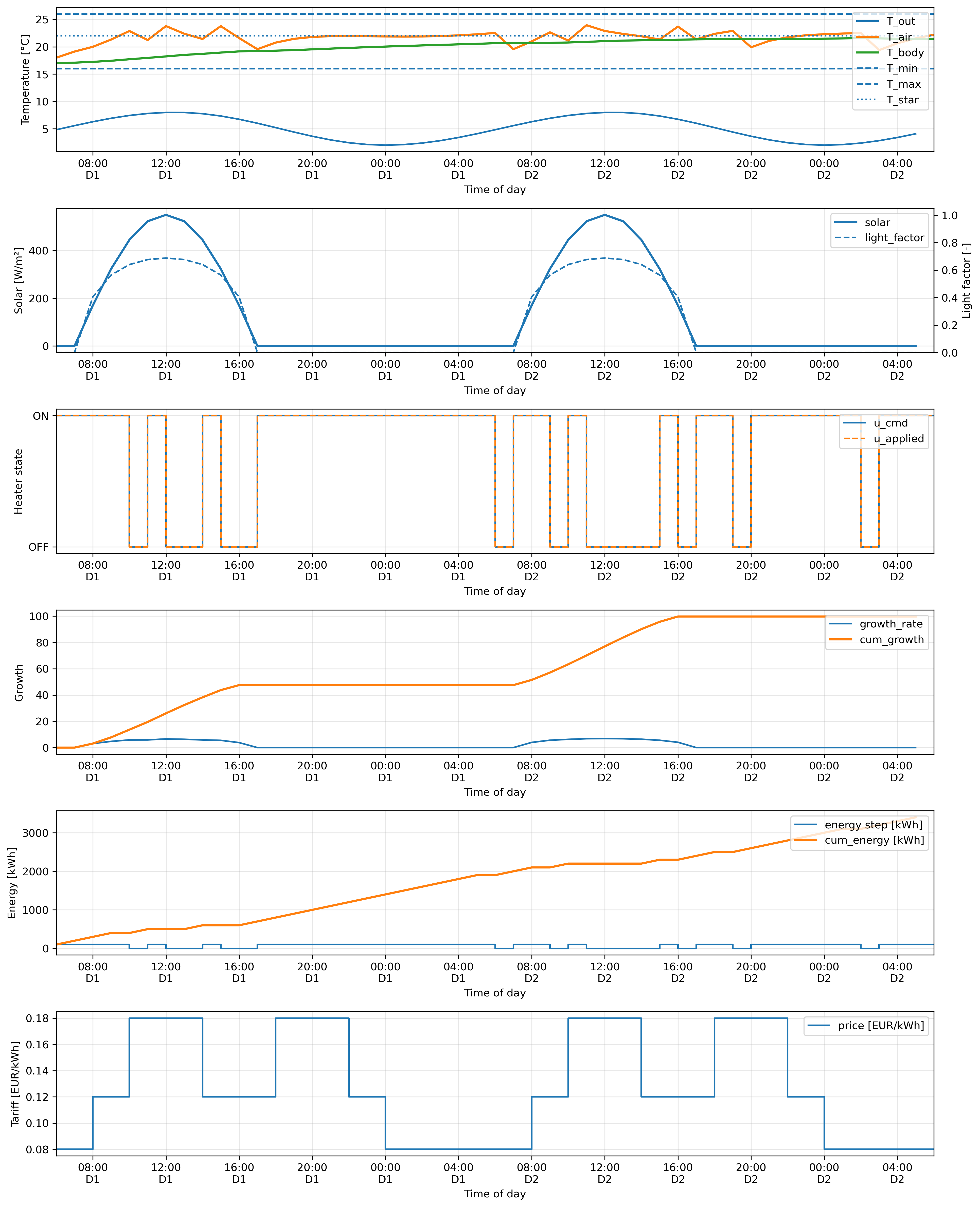
The benchmark is structured as a single-actuator (binary heater) model-predictive-control problem over a 24-hour horizon at Δt=1 h. The plant is a discrete-time linear two-state thermal system — air temperature T_air,k and a slower body/canopy temperature T_body,k — driven by outdoor temperature, a half-sine solar radiation profile, and the heater. A growth proxy g_k = L_k(g_max − η(T_grow,k − T∗)²) penalises departures from a preferred growth temperature T∗=22°C, scaled by a saturating light factor. Energy use is metered as E_k = P_heateru_kΔt, electricity cost as C_k = λ_Ep_kE_k, switching cost is λ_S per heater toggle, and the temperature trajectory is constrained to 16–26°C.

Section 3 unrolls the discrete-time dynamics, writes the state as an affine function x_k = x̅_k + ∑_tΓ_k,tu_t of the binary heater sequence, and substitutes into the growth and feasibility expressions. Because T_grow,k is affine in u, the squared growth deviation is quadratic in u; the energy and switching terms are linear-quadratic; and the bounds enter as two one-sided quadratic penalties with lower- and upper-slack binary registers. The authors note explicitly (and somewhat unusually for QUBO benchmark papers) that they use both lower and upper slacks even though only one is required, doubling the slack footprint and the coupler-graph density — this design choice is called out as a likely contributor to the dense BQM and is flagged for future improvement.

Section 4 spells out the solver protocol with a level of reproducibility detail that is rare for D-Wave benchmarks: explicit dwave-system v1.34.0, dimod v0.12.21, dwave-samplers v1.7.0 versions; explicit annealing time (20 µs); the solver Advantage2_system1; the hybrid solver tag hybrid_binary_quadratic_model_version2p. The paper also flags the limitation that EmbeddingComposite’s default chain strength was used and chain-break statistics were not recorded — an honest disclaimer that the QPU degradation at H=14 cannot be cleanly attributed to logical-problem difficulty vs. embedding quality.

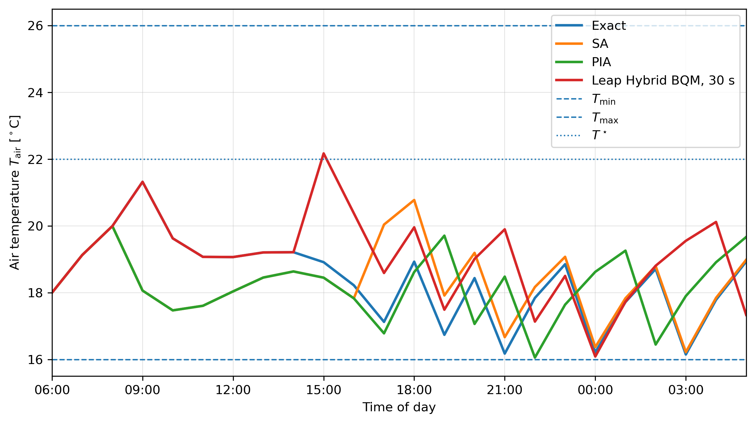
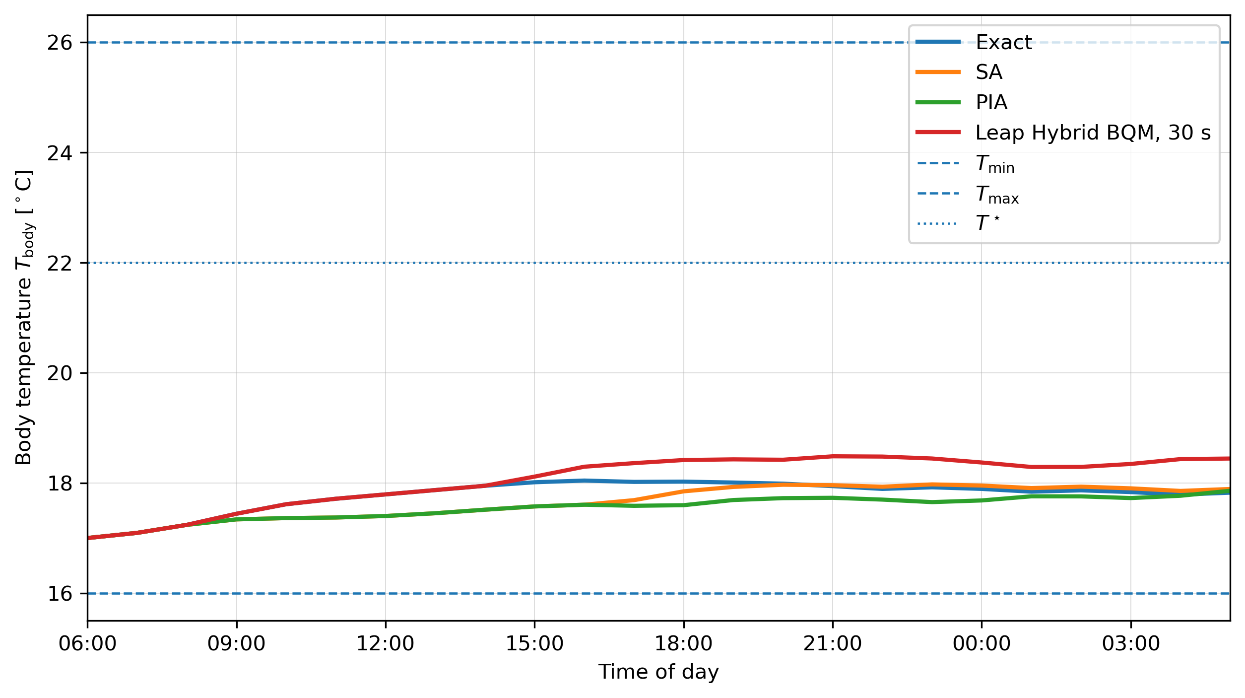
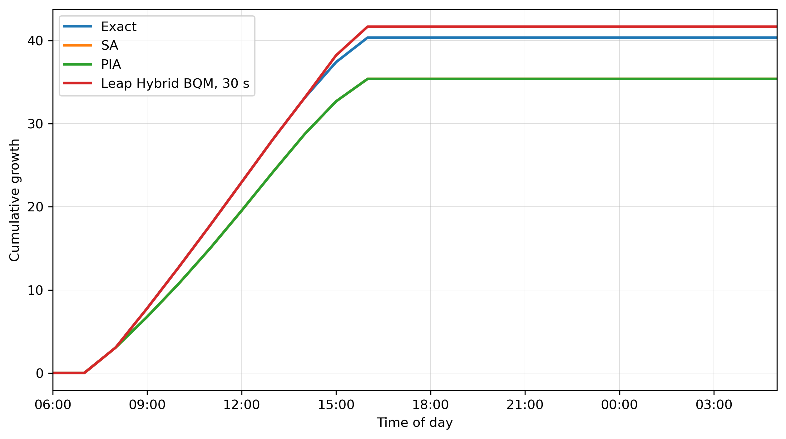
Section 5’s results are the headline. At H=24, exact enumeration (~2²⁴~17M schedules, 1 028 s wall clock) gives J=−145.14. SA achieves −150.11 best and −161.60 mean in 31.84 s; PIA matches it in 3.6 s (best −149.11, mean −169.94). The Leap Hybrid BQM at 30 s is markedly worse: best −174.32, mean −203.84, and only 7 of 10 runs return a feasible decoded schedule. Increasing the requested hybrid time to 60 s actually decreases the feasible-run rate to 2/10 (Table 3). The authors carefully caveat that this non-monotonicity could be a sample-size artefact (10 submissions per setting) and that the hybrid solver is not designed for H=24 problem sizes — an important honest framing. Crucially, when the hybrid solution is feasible, it tends to over-heat (best hybrid uses 1 300 kWh, 13 heater-on intervals, vs. exact 1 100 kWh, 11), driving growth slightly above exact (41.68 vs. 40.36) but objective well below.

On the reduced direct-QPU scan (Section 5, Table 4), the exact-hit rate cleanly degrades with horizon: H=10 = 5/10, H=12 = 2/10, H=14 = 0/10, while SA and PIA stay essentially at the exact optimum (PIA mean −6.79 ± 0.38 at H=12, −36.74 ± 2.33 at H=14). The mean QPU performance also shows much larger variance (±12.71, ±18.07, ±23.38) than SA/PIA. Importantly, all QPU samples remain feasible — the degradation is in optimality, not constraint satisfaction. This is a cleaner story than typical D-Wave benchmarks, which often blur feasibility-failure into “quantum failure.”

Section 5’s discussion is unusually honest about why the hybrid solver underperforms: penalty scaling (A_bound=120 chosen empirically), the dense coupling structure from the rollout dynamics, the mismatch between internal BQM energy and decoded simulator objective, and the doubled-slack representation. Section 6 lists limitations clearly — coarse 1-hour sampling, single binary actuator, no manual chain-strength tuning, no embedding-quality logging — in a way that pre-empts reviewer push-back. Section 7’s conclusion repeats the no-quantum-advantage framing and points to multi-day horizons (H=72, H=168) plus richer multi-actuator models as next steps.

Figures

Toy model overview — Figure 1. Overview of the greenhouse toy-model simulator over the benchmark horizon, with the horizontal axis expressed as clock time. From top to bottom, the panels show: (i) the thermal trajectories T_out, T_air, and T_body together with the bounds T_min, T_max, and the reference temperature T∗; (ii) the prescribed solar radiation and the derived light factor; (iii) the heater control variable u_k∈{0,1}, shown for both commanded and applied heater signals; (iv) the instantaneous growth proxy and cumulative growth; (v) the interval energy use and cumulative energy consumption; and (vi) the electricity price tariff used to weight energy consumption over the day.

Air temperature trajectories — Figure 2. Best feasible air-temperature trajectories for the H=24 benchmark. Only the best feasible decoded solution of each solver workflow is shown to keep the comparison readable. The admissible interval is defined by T_min=16°C and T_max=26°C.

Body temperature trajectories — Figure 3. Body-temperature trajectories for the best feasible decoded solutions of the H=24 benchmark. The body temperature is smoother than the air temperature and mainly serves as a secondary diagnostic of the two-state thermal model.

Figure 4. Cumulative growth proxy for the best feasible decoded solutions of the H=24 benchmark. The figure is provided as an additional diagnostic because the main growth–energy–switching trade-off is reported quantitatively in Table 2.

Citations to Yuan's papers

No direct citation to any of Y1–Y6 found in bibliography.

Overlap with Y1–Y6

Y3 (QAOA DGMVP portfolio, QST 2026) — closest conclusion overlap. Y3 concluded that thermal relaxation precludes quantum advantage on a discrete-binary global minimum variance portfolio, with the shot-noise-only regime showing favourable scaling. This paper concludes from a different angle — quantum annealing on D-Wave Advantage2 rather than gate-based QAOA on IBM — that current quantum/hybrid annealing workflows do not beat strong classical SA baselines on a structured constrained binary QUBO. Different hardware family, same end-state. The paper’s decoded-simulator-side evaluation methodology (separating raw BQM energy from physical objective) is also a methodology Yuan could borrow for future portfolio-QAOA benchmarks.
Y2 (quasi-binary QAOA portfolio) — scope overlap on the binary-encoded constrained-optimisation framing. Y2 uses ~2 log₂(U−L+1) qubits per variable with a constraint-preserving hard mixer (no penalty); this paper uses M=6 binary slack bits per inequality with a penalty term. The contrast (hard-mixer encoding vs. penalty-slack encoding) is exactly the design axis Y2 argues against, and this paper’s explicit complaint that the doubled lower/upper-bound slack registers inflate BQM density into 4 596 couplers is direct empirical evidence for Y2’s thesis.
Y4 (Grover + ADMM cardinality-constrained BO) — scope overlap on constrained binary optimisation, but no method overlap (Y4 is gate-model Grover, this is annealing). The relevant connection is that Y4’s ADMM hybrid pre-processes the cardinality constraint classically, which is conceptually analogous to this paper’s argument that better inequality encoding would shrink the BQM.
Y1, Y5, Y6 — no substantive overlap.

Recommended action for Yuan

Cite in the next Y3 follow-up. This paper is a near-perfect external corroboration of Y3’s “no quantum advantage in the thermal regime” finding, on a completely different hardware stack (D-Wave annealing) and problem (control QUBO rather than portfolio). It strengthens any review or perspective piece Yuan might write on the QAOA-portfolio-vs-quantum-annealing landscape.
Borrow the decoded-simulator-side evaluation protocol. The clean separation of raw BQM energy vs. decoded physical objective vs. feasibility violation count is methodologically clean and would be a useful addition to Y3-style portfolio benchmarks — especially if Yuan continues comparing QAOA against simulated-annealing baselines.
Adapt the penalty-vs-hard-mixer comparison. The paper’s honest discussion of how penalty-encoded inequality constraints inflate coupler density and degrade hybrid-solver performance is the kind of evidence Y2’s hard-mixer thesis is built on. Worth surfacing in any follow-up paper comparing quasi-binary encoding against D-Wave-style penalty encoding on the same problem.