Mechanism of Efficacy in QAOA for Random k-SAT: From Adiabatic Manifold to Sublinear Parameter Optimization

Mingyou Wu, Hanwu Chen (Southeast University) · arXiv:2605.20288 · submitted 2026-05-21 · score 8/10 (HIGH)

Abstract

The Quantum Approximate Optimization Algorithm (QAOA) is a leading candidate for demonstrating quantum advantage on near-term devices, yet the physical origins of its efficacy remain poorly understood. In this work, we study QAOA for random k-SAT problems within a universal-mixer k-local search framework, establishing a formal correspondence between adiabatic state transfer and the QAOA ansatz. This correspondence yields a rigorous performance guarantee for random instances with clause density m = 𝒪(n^1+ε) and circuit depth Θ(n²). We further investigate the NISQ regime with shallow circuits of depth p = 𝒪(n). Surprisingly, the optimal parameters do not become stochastic under depth compression, but instead remain confined to a structured low-dimensional region, which we identify as a smooth adiabatic manifold. Numerical evidence indicates that this manifold persists across different circuit depths and arises from the variational suppression of adiabatic leakage. Based on this structure, we propose the smooth adiabatic-manifold parameterization (SAMP) strategy, transforming parameter optimization from an unstructured high-dimensional search into a guided refinement process. Numerical experiments on random 3-SAT instances show that SAMP achieves sublinear optimization scaling with circuit depth while providing robust zero-cost initialization for deep circuits.

Executive summary

Wu and Chen establish a rigorous adiabatic interpretation of QAOA for random k-SAT and exploit it to slash the parameter-tuning cost. At quadratic depth p = Θ(n²) they prove QAOA solves typical max-k-SSAT instances with probability 1 − 𝒪(erfc(n^δ/2)). At NISQ-relevant linear depth p = 𝒪(n) the optimal parameters do not scatter; they concentrate on a smooth two-parameter (θ, ρ) manifold with θ* ≈ π/4 and ρ* growing linearly in n. They turn this geometric observation into an algorithm — SAMP — that reparameterises (γ, β) in (τ, θ) coordinates and uses hierarchical doubling of the degrees of freedom to optimise. Empirically, SAMP achieves sublinear (effectively 𝒪(log p)) optimization cost while matching or beating FOURIER and TQA initialisation on 100 random 3-SAT instances up to n = 20. For Yuan, this is a strong methodological neighbour to Y1 (warm-starting via structural priors), Y3 (layerwise optimisation alternatives), and the broader QAOA parameter-tuning programme.

Main contribution

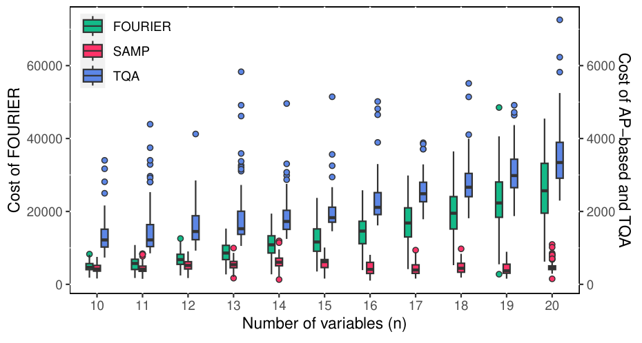
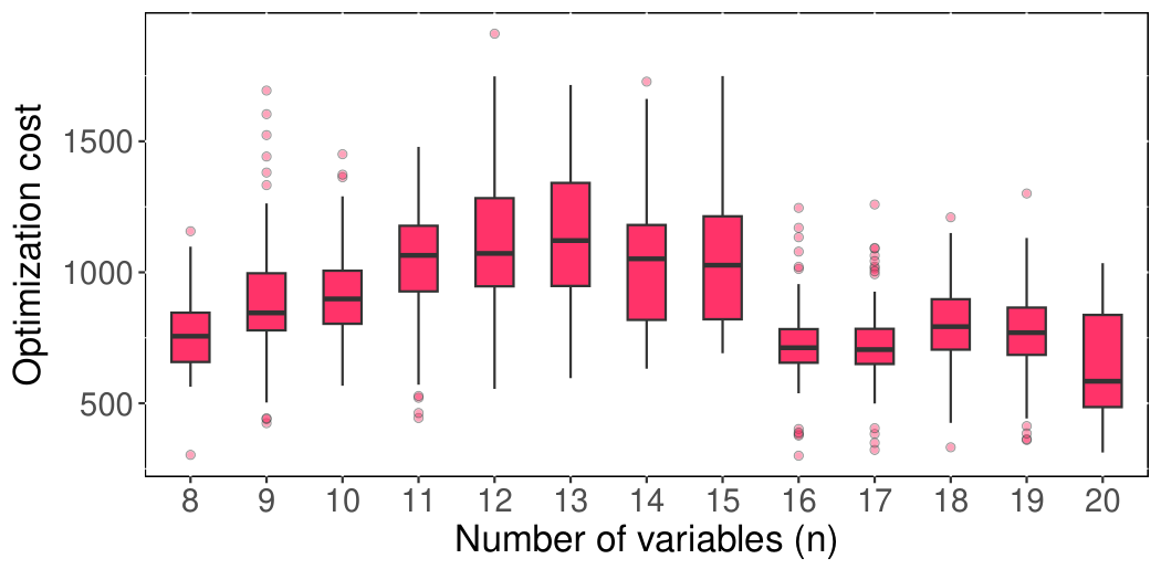
The paper has two layers. First, a theoretical result: by introducing max-k-SSAT (a satisfiable-only restriction of max-k-SAT preserving NP-hardness, Lemma 1) and a universal-mixer k-local search formulation, the authors show QAOA's ansatz emerges as a Trotter discretisation of an adiabatic k-local search. Theorem (Sec III) gives: for p = Θ(n²) and m = Θ(n^1+ε), success probability 1 − 𝒪(erfc(n^δ/2)). Second, an algorithmic result: at p = 𝒪(n), the optimal QAOA parameters lie on a smooth manifold parameterised by (θ, ρ); reparameterising into (τ_d, θ_d) coordinates with γ_d = (2πd/(p+1))τ_dsinθ_d, β_d = (2π(p−d+1)/(p+1))τ_dcosθ_d (Eq. 21) and refining the degree of freedom by doubling (Algorithm 2) gives logarithmic optimization stages. The headline figure: optimisation cost goes from ~300 (n=4) to ~546 (n=20), versus FOURIER's growth from 4854 to 26122 over the same range — about a 50× reduction at n=20.

Key theorems / lemmas / algorithms

Lemma 1 (problem reduction): if max-k-SSAT is solvable in 𝒪(f(n)) time, so is the k-SAT decision problem — preserves NP-hardness while admitting an optimisation framing.
Theorem 3.1 (Section III, p = Θ(n²) guarantee): for random instances from F_s(n, m, k) with m = Θ(n^1+ε), the universal-mixer k-local search variant of QAOA solves typical instances with success probability 1 − 𝒪(erfc(n^δ/2)).
Lemma (spectral gap, Lemma 4.2): the system Hamiltonian 𝓗_k(s) has spectral gap Θ(n⁻¹) — the basis for argued robustness of compressed-depth evolution.
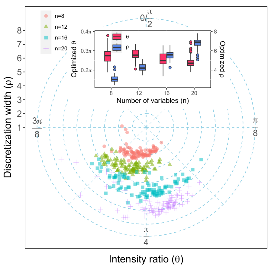
Smooth Adiabatic Manifold (definition, Sec IV.B): the low-dimensional submanifold of (γ, β) on which optimal QAOA parameters concentrate even at p = 𝒪(n); empirically θ* ≈ π/4, ρ* ∝ n.
Adiabatic-manifold reparameterisation (Eq. 21, Sec IV.C): γ_d = (2πd/(p+1))τ_dsinθ_d; β_d = (2π(p−d+1)/(p+1))τ_dcosθ_d.
Algorithm 2 (hierarchical refinement): initialise (θ₀, τ₀) = (π/4, √2), rescale Hamiltonians, then for T_u ≤ ⌊log₂ p⌋ iterations, double the number of sampling points via cubic-spline interpolation and re-optimise.

Detailed walkthrough

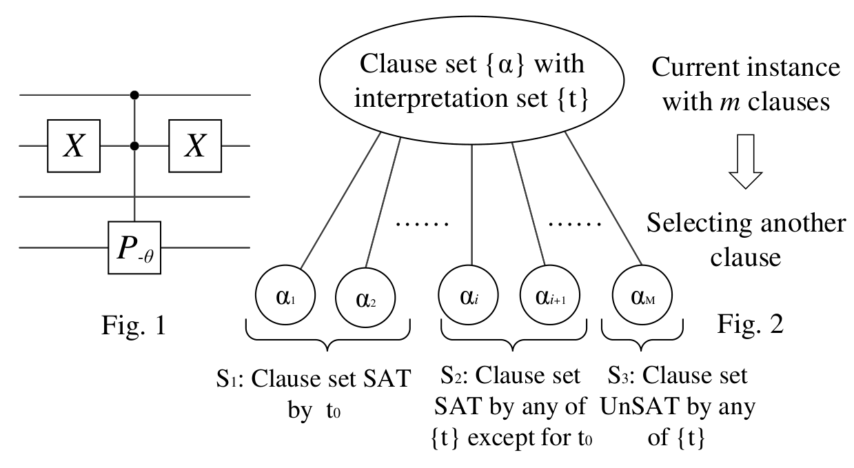
Section II reduces k-SAT to max-k-SSAT and analyses statistical properties of the resulting problem Hamiltonian. The key observation is that random satisfiable instances concentrate sharply around an effective k-local search problem — this is what lets the adiabatic argument bite.

Section III (adiabatic origin) introduces a universal-mixer generalisation of k-local quantum search and shows QAOA's standard ansatz emerges as a special case. The authors then prove that at p = Θ(n²) — the canonical adiabatic depth — the algorithm enjoys a rigorous success-probability guarantee for typical instances. The "universal-mixer" framing matters: it generalises Grover-style mixers and connects QAOA to adiabatic computation more cleanly than prior analyses on regular MaxCut.

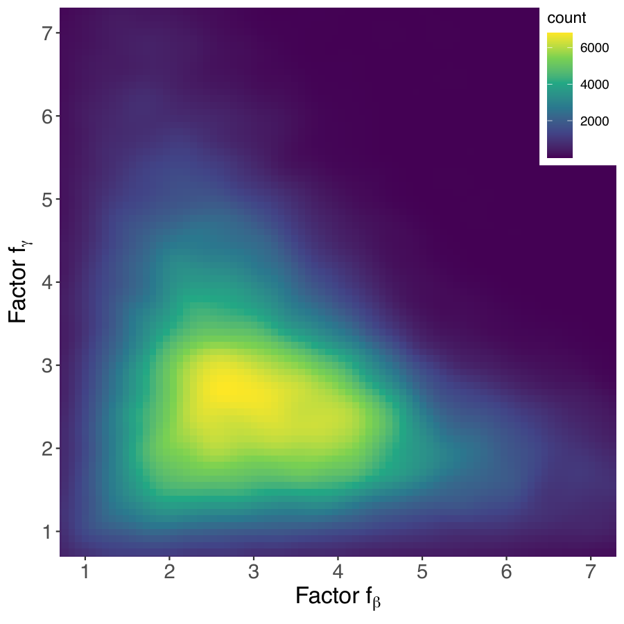
Section IV.A–B (manifold discovery) is the empirical heart of the paper. Starting from a linear schedule with a single time-rescaling parameter ρ (Eq. 12), the authors observe that the success amplitude on n = 16, 18, 20 instances peaks sharply at specific (n-dependent) ρ values (Table I — at n = 20, peak amplitude 0.918 near ρ = 7.5). They then add a second degree of freedom (f_γ, f_β) controlling relative Hamiltonian strengths (Eq. 13) and find a clear diagonal ridge of high success probability (Fig. fig_exp4ng). Factoring out the global energy scale, this collapses to a single angle θ with θ* ≈ π/4 in polar coordinates (Fig. fig_exp4id), with the scaling parameter ρ* growing linearly in n. They name this region the smooth adiabatic manifold and argue it inherits its smoothness from the spectral concentration of the problem Hamiltonian under F_s.

Section IV.C–D (reparameterisation and refinement) turns the geometric observation into an optimisation strategy. The reparameterisation γ_d/β_d = (linear envelope)·τ_d·{sin,cos}θ_d bakes the "linear-schedule × rotation angle" structure into the parameter space. The hierarchical refinement (Algorithm 2) starts with one degree of freedom, optimises, then doubles the degrees by cubic-spline interpolation, and re-optimises — log₂(p) stages total. This is conceptually similar to FOURIER (Zhou 2020) but FOURIER grows degrees-of-freedom linearly, costing 𝒪(n) outer iterations; SAMP's geometric doubling gives 𝒪(log n).

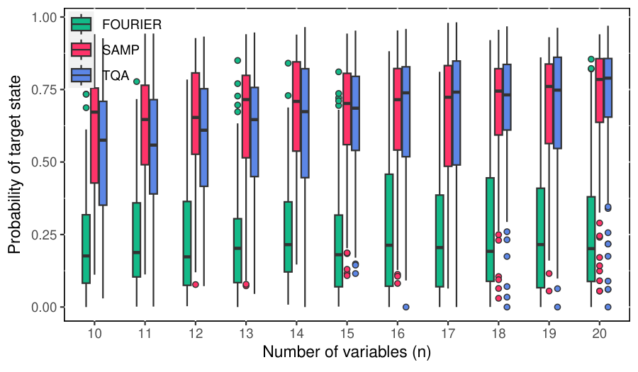
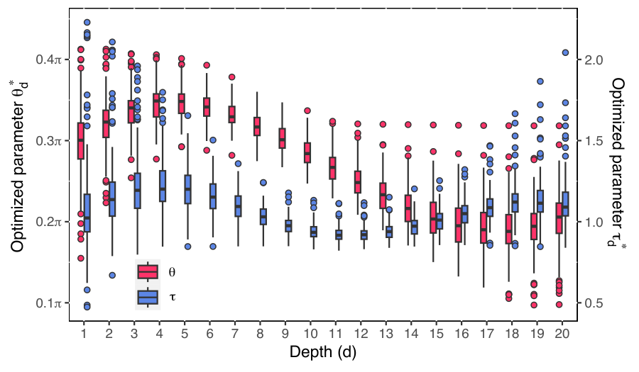
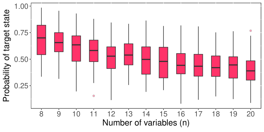
Section V (numerical results) benchmarks on 100 random instances per n ∈ [10, 20] near the satisfiability threshold, with QAOA depth p = n. The success-probability distributions (Fig. fig_SAMP_com1a) show SAMP ≈ TQA > FOURIER. The optimisation-cost results (Fig. fig_SAMP_com1b) are the key takeaway: FOURIER ≈ 4854→26122 (slightly worse than n²), TQA ≈ 1327→3523 (linear with a precomputation upfront), SAMP ≈ 300→546 (sublinear, effectively log p). Table II resolves the cost scaling by ⌊log₂ p⌋ — the cost increments are nearly constant across each log-interval. Fig. fig_exp6para shows the optimised (θ_d, τ_d) profiles are smooth trigonometric-looking curves, with max τ / min τ < 2, consistent with the manifold smoothness hypothesis. Appendix shows the same machinery extends to Erdős–Rényi MaxCut at density 0.5, suggesting generality beyond SAT.

Section VI (discussion) outlines the path to general combinatorial problems: derive a random model, characterise the problem-Hamiltonian eigenvalue distribution, normalise, and reuse the (θ, τ) manifold parameterisation. The framework is genuinely portable — exactly the kind of structural prior Yuan's iterative warm-start (Y1) builds on top of.

Figures

Performance comparison (success probability) — Distribution of success probabilities for FOURIER (green), SAMP (red), and TQA (blue) over 100 random instances from F_s(n, m_n*, 3) with 10 ≤ n ≤ 20.

Performance comparison (optimisation cost, dual y-axis) — same 100 instances; FOURIER ≈ 𝒪(n²), TQA ≈ 𝒪(n), SAMP sublinear.

Distribution of measurement counts for the target state |t⟩. For each (f_γ, f_β) pair, 10,000 shots on a random instance from F_s(12, m, 3) with p = n. The diagonal ridge f_γ ≈ f_β visualises the adiabatic manifold.

Distribution of optimal (θ*, ρ*) for 100 random instances of F_s(n, m, 3) in polar coordinates: n = 8 (red ○), 12 (green △), 16 (blue □), 20 (purple ×). θ* clusters around π/4; ρ* increases approximately linearly with n.

Distribution of optimised (θ*, τ*) for 100 random instances in F_s(20, m_n*, 3) — red (left) and blue (right). The optimised parameters exhibit superior continuity reminiscent of trigonometric functions; even outliers stay close to adjacent values.

Distribution of success probabilities for SAMP on random Erdős–Rényi MaxCut instances with edge density 0.5, n = 8 to 20.

Distribution of optimisation costs for SAMP on the same Erdős–Rényi MaxCut instances — comparable cost to the 3-SAT setting.

Clause selection process in generating a random k-SAT instance. F(n,m,k) samples uniformly; F_s(n,m,k) restricts to clauses satisfied by at least one assignment in {t}; F_f(n,m,k) restricts to clauses satisfied by a fixed t₀.

Citations to Yuan's papers

No direct citation to any of Y1–Y6 found in bibliography.

Overlap with Y1–Y6

Y1 (iterative warm-started QAOA, MaxCut, DGMVP scaling): very close — both papers exploit structural priors on QAOA parameter landscapes to bypass barren-plateau-style optimisation. Y1's iterative warm-start is essentially a problem-instance-dependent initialisation; SAMP is a problem-class initialisation grounded in adiabatic geometry. The two are complementary: SAMP could serve as the initial point for Y1's iterative loop, and Y1's measurement-derived corrections could refine SAMP's first-stage (τ, θ) optimum. The MaxCut extension in Appendix C of this paper is exactly the regime Y1 studied.
Y2 (quasi-binary encoding + hard mixer, portfolio): orthogonal mechanism — Y2 reduces qubit count and enforces feasibility via mixer design; SAMP is mixer-agnostic but reduces classical optimisation cost. Combining them is straightforward in principle.
Y3 (QAOA DGMVP portfolio, layerwise optimisation): directly comparable on the "QAOA parameter optimisation strategy" axis. Y3 found dual annealing + layerwise was the most robust optimiser for portfolio QAOA; SAMP is a competitor that — if it generalises to portfolio Hamiltonians — could replace the layerwise pipeline. A direct head-to-head on the DGMVP test bed from Y3 would be informative; the prerequisites (random portfolio Hamiltonian model, energy normalisation, manifold structure check) are explicitly listed in Sec. VI.A of this paper.
Y4 (Grover + ADMM cardinality): the universal-mixer k-local search framework here generalises Grover; the depth Θ(n²) guarantee at superlinear clause density "far exceeds the guarantees derived from unstructured Grover-type search" (intro). For Yuan's Grover work, this is a useful theoretical comparator.
Y5 (Pauli-sparse Gibbs SDP): no overlap.
Y6 (PBR / hardware): no overlap.

Recommended action for Yuan

Read deeper: Sec. IV.C (reparameterisation Eq. 21) and Algorithm 2 — this is the most directly implementable piece. The mapping from a generic linear adiabatic schedule to (τ, θ) coordinates with hierarchical doubling is a few dozen lines of code and should be benchmarkable against Y3's dual-annealing pipeline on DGMVP instances within a day or two.
Implement for comparison: run SAMP on Y3's portfolio QAOA test bed at p = 𝒪(n) and report whether the sublinear scaling holds for portfolio Hamiltonians. If yes, this is a candidate replacement for Y3's optimiser; if no, the comparison itself is publishable.
Cite in next iterative-warm-start follow-up: the smooth-adiabatic-manifold concept is a clean way to motivate why warm-starting works at all — Y1's framing currently lacks this structural prior.
Discuss with Barnes: the Θ(n²) success-probability bound (vs. Grover's quadratic) is the kind of structural-vs-unstructured speedup result the Y1–Y4 lineage will eventually need to engage with.