Breaking QAOA's Fixed Target Hamiltonian Barrier: A Fully Connected Quantum Boltzmann Machine via Bilevel Optimization

Liu Jun (Hunan University of Finance and Economics) · arXiv:2605.07473 · submitted 2026-05-11 · score 8/10

Abstract

To overcome the limitations of classical partially connected Boltzmann machines and mainstream quantum Boltzmann machines (QBMs), this work extends the conventional circuit of the quantum approximate optimization algorithm (QAOA) to a bilevel optimization architecture and proposes a fully connected QBM. Specifically, this work breaks the constraint that the target Hamiltonian in standard QAOA circuits is fixed by setting its structural parameters as optimizable variables, which are used to map the energy function parameters of the fully connected Boltzmann machine. The inner-loop training simulates positive phase energy minimization based on the computational process of the conventional QAOA circuit, whereas the outer-loop training simulates negative phase contrastive divergence learning by optimizing the structural parameters of the target Hamiltonian. … The model exhibits superior performance using only a single layer (p=1) in the QAOA circuit, with an average probability of 0.9559 in measuring the target quantum state under noiseless conditions. … Under the typical noise level of current mainstream commercial quantum computing devices, the average probability of measuring the target quantum state reaches 0.6047; when the noise rises to a more stringent level with doubled intensity, this probability remains at 0.3859.

Executive summary

This is a single-author paper that proposes a structurally simple but conceptually consequential variant of QAOA: rather than treating the cost Hamiltonian H_1 = Σ b_i Z_i + Σ w_ij Z_i Z_j as fixed and optimizing only the variational angles (γ, β), the author treats (b_i, w_ij) as outer-loop learnable parameters too. Inner loop: standard QAOA energy minimization over (β, γ) at fixed Hamiltonian (positive phase / energy minimization initialization). Outer loop: parameter-shift gradient descent on (b_i, w_ij) under a mean-squared-error-as-Hamiltonian loss H_2 against a user-specified target distribution (negative phase / contrastive divergence). The paper demonstrates this on a 4-qubit toy distribution (single-point target |1001⟩) and a 4-block × 40-block image-generation task ("qubit" pixel art) under depolarizing noise of 0.5%/2% and 1%/4% single/two-qubit gate error rates. For Yuan, this is a method-overlap hit on Y1's "structural parameter scheduling" theme, with a clean noise-robustness scan on a generative use of QAOA.

Main contribution

The architectural contribution is the bilevel QAOA loop. Inner loop minimizes ⟨H_1⟩ over (β, γ) by parameter-shift gradient descent; outer loop minimizes ⟨H_2⟩ = (1/2^N) Σ (P(i) − P_T(i))² over the Hamiltonian's structural parameters (b_i, w_ij) by the same parameter-shift rule. The author argues that this turns a vanilla QAOA into a fully connected QBM: the unrestricted topology preserves higher-order correlations that RBM/DBM bipartite restrictions discard, while the quantum measurement directly delivers normalized basis-state probabilities without ever computing the partition function. The experimental claims are p=1 sufficiency, strong noise robustness at NISQ-typical and 2× NISQ-typical depolarizing rates, and successful block-by-block reconstruction of an 8×20 image with only 10 shots per 4-qubit block.

Key theorems / lemmas / algorithms

Bilevel ansatz: |ψ⟩ = Π_{k=1..p} e^{iβ_k H_0} e^{iγ_k H_1(b,w)} |+⟩^{⊗N}, with H_1's coefficients also optimizable.
MSE-as-Hamiltonian (Eq. 18–19): H_2 = (1/2^N) Σ_i (M_i ρ_ψ M_i − 2P_T(i) M_i + P_T(i)² I) with M_i = |i⟩⟨i|, and the identity ⟨ψ|H_2|ψ⟩ = MSE(P, P_T).
Parameter-shift gradients (Eqs. 16, 17, 20, 21) for all four sets of variables (β_k, γ_k, b_i, w_ij), using the standard ±π/2 rule.
Sequential bilevel scheduling: in each outer iteration, run inner loop to convergence then take outer steps to convergence. The author reports this beats a nested scheme in both convergence and resource usage, but provides no formal proof.
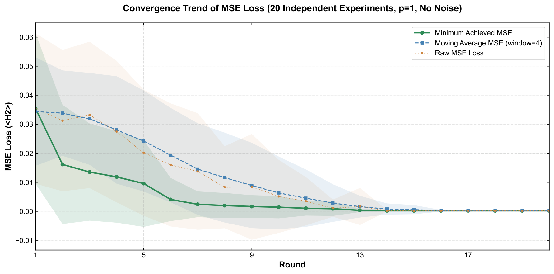
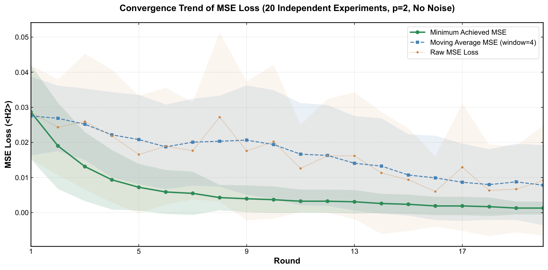
Experimental claim 1 (noiseless): for the target |1001⟩, p=1 yields P(target) = 0.9559 ± 0.0342 across 20 runs; p=2 yields 0.9009 ± 0.0664 — so deeper is worse, attributed to more gates → more compounded noise. This is a notable empirical claim and worth scrutinizing.
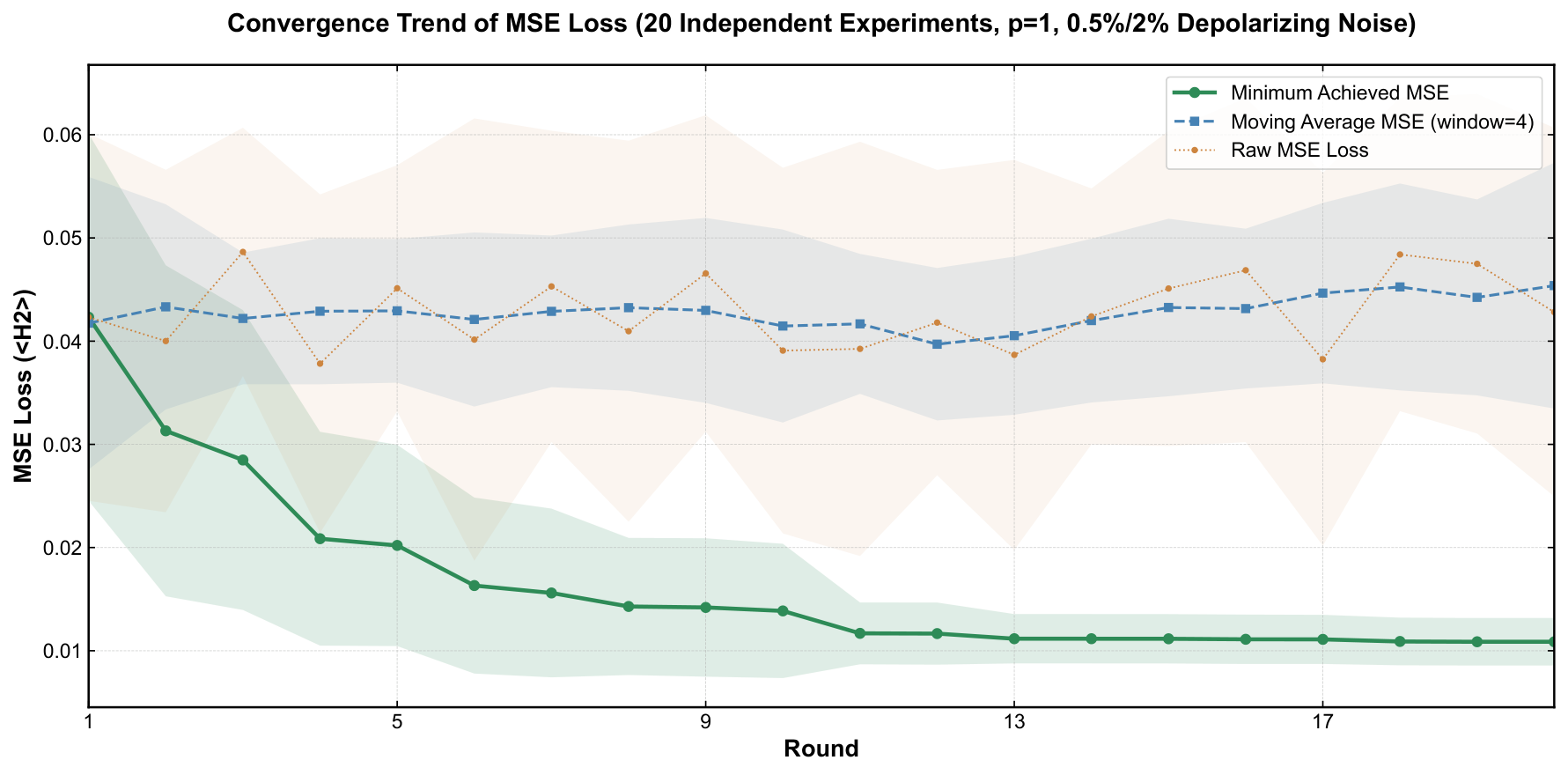
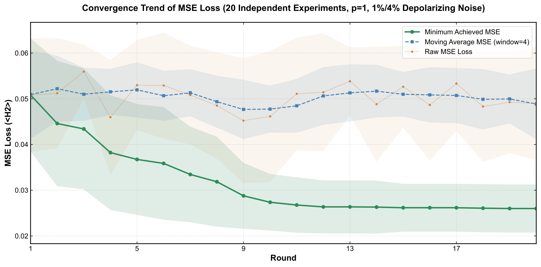
Experimental claim 2 (NISQ noise): at 0.5%/2% gate-error rates the target probability holds at 0.6047 ± 0.0418; at 1%/4% (doubled) it is 0.3859 ± 0.0537 — still the rank-1 outcome by several factors over runner-up.
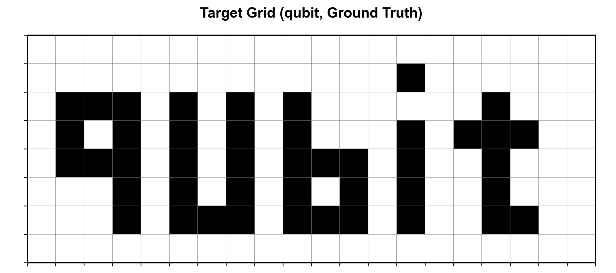
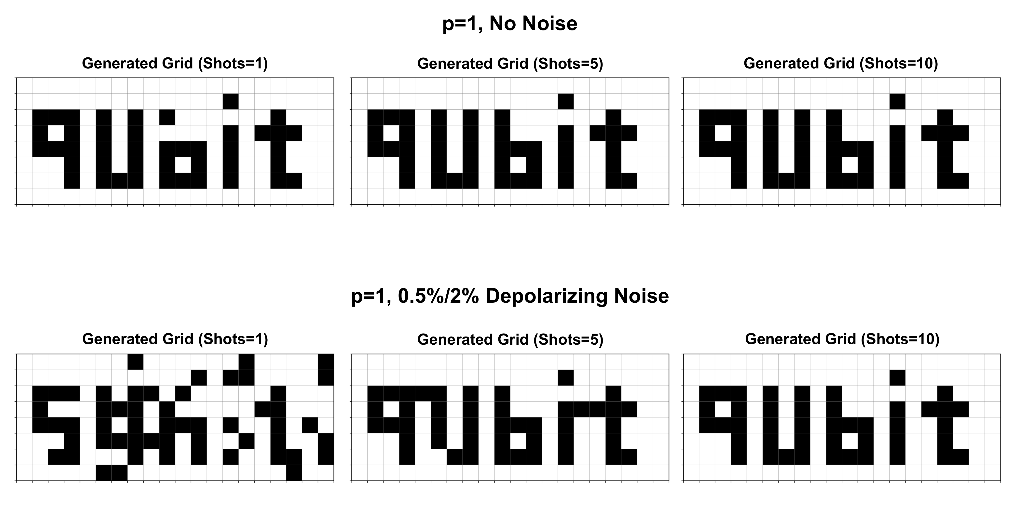
Experimental claim 3 (image generation): 8×20 pixel "qubit" image reconstructed block-by-block (40 × 2×2 blocks) at p=1 with only 10 measurement shots per block.

Detailed walkthrough

Section 2 is a textbook setup of the classical fully connected Boltzmann machine — energy E(s; Θ) = Σ b_i x_i + Σ w_ij x_i x_j, probability P(s; Θ) ∝ exp(−E(s; Θ)), partition function Z, KL-divergence loss, and Gibbs-sampling-based parameter updates — used to motivate why classical implementation of the fully connected (rather than restricted) BM is intractable: Z sums over 2^N states and Gibbs sweeps scale as O(G·N²).

Section 3 is the bilevel quantum scheme. The energy function is mapped to H_1 = Σ b_i σ_z^i + Σ w_ij σ_z^i σ_z^j — i.e., a generic Ising Hamiltonian where the coefficients are now learnable. Inner-loop training is identical to standard QAOA: run the circuit at current (b, w), measure ⟨H_1⟩, parameter-shift-differentiate w.r.t. (β, γ), descend. Outer-loop training is more interesting: the loss is the MSE between the QAOA output distribution and a user-specified target. The author works out (Eq. 18 onward) that this MSE can be written as the expectation of a Hermitian Hamiltonian H_2 in the QAOA-prepared state, and crucially that the parameter-shift rule applies to gradients of ⟨H_2⟩ with respect to the Hamiltonian's own coefficients (b_i, w_ij) — because those coefficients appear in the unitary e^{iγ_k H_1} as linear factors, the ±π/2 trick still works after a per-term decomposition.

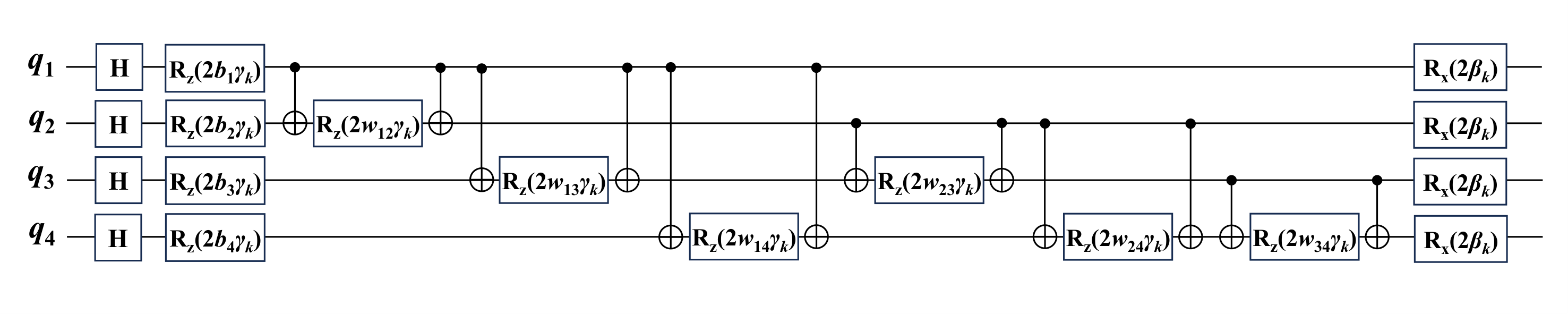
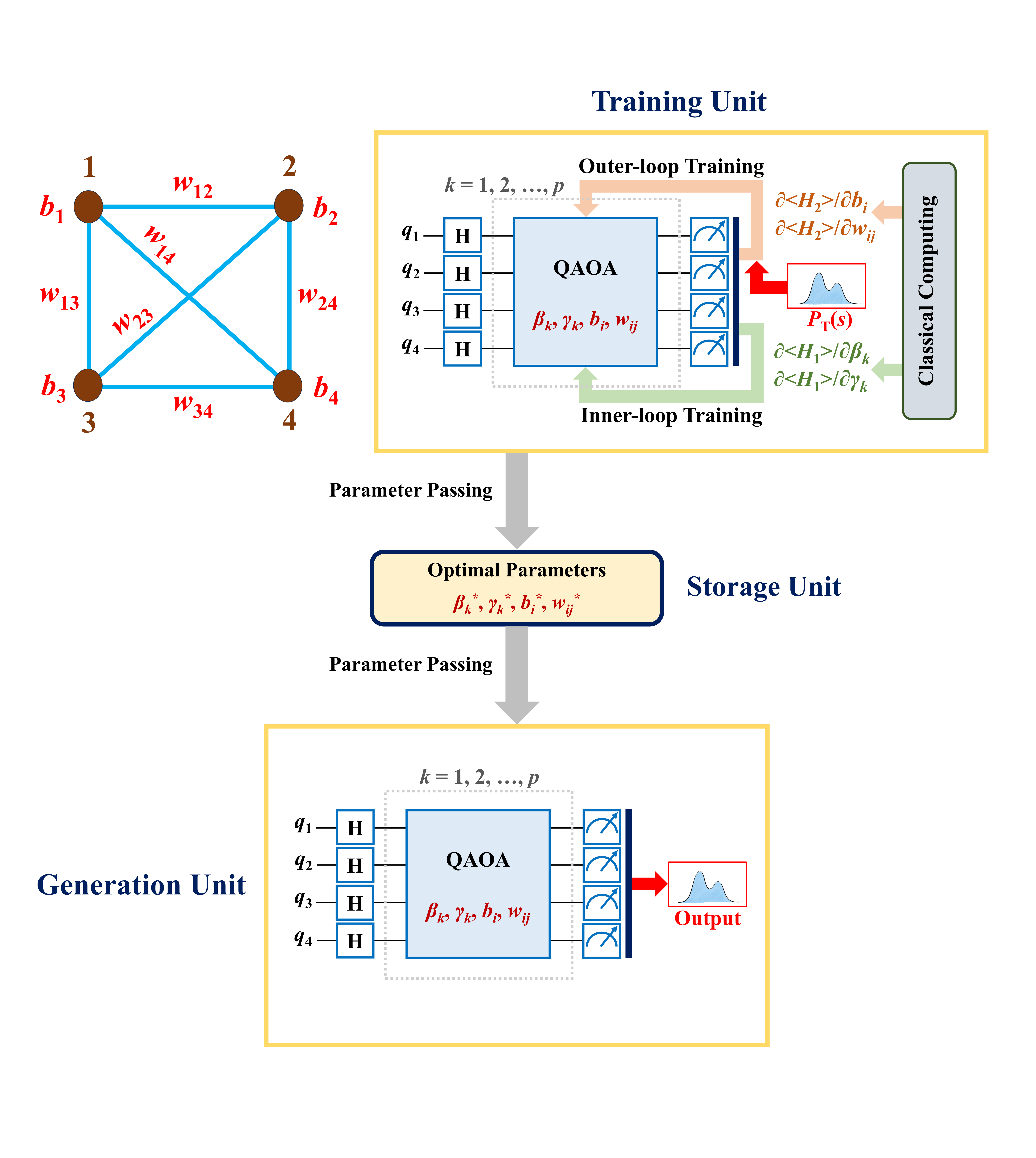
Section 4 instantiates the scheme for N=4. The circuit (Fig. 1, the per-layer schematic; Fig. 2, the full training/generation/storage three-unit architecture) is the standard QAOA: Hadamard initial state, alternating e^{iγ H_1} and e^{iβ H_0} with H_0 = Σ σ_x^i. The target distribution is a one-hot (Kronecker) over a single 4-bit string.

Section 5 reports the experiments on PennyLane. The author tests p=1 vs p=2 under noiseless conditions, finds p=1 is empirically better, and pins this on circuit-depth-driven complexity sensitivity. This is a noteworthy finding: in the literature p=2 typically dominates p=1 for QAOA approximation ratios on combinatorial problems, but in this toy generative task the target is a single Kronecker delta and a single layer of cost rotations followed by a single layer of mixing rotations seems to be enough expressive power, while p=2 doubles the parameter count and (apparently) makes the variational landscape harder to navigate to the global optimum. The noise-robustness experiments are then run at p=1 only, with depolarizing channels of the stated rates. The image-generation experiment uses 40 independent 4-qubit blocks, each trained to a one-hot target derived from a 2×2 patch of the 8×20 "qubit" word image. The reconstruction at 10 shots per block under noise is qualitatively convincing as displayed in Fig. 8.

A few caveats. The 4-qubit demonstration leaves the actual scaling story untested — the bilevel optimization adds O(N²) outer parameters on top of the existing O(p) inner parameters, so the outer-loop gradient cost via parameter-shift is O(N² × inner-loop-cost). The block-by-block image trick sidesteps this by keeping each block at 4 qubits, but a single fully connected QBM at, say, N=20 would be a more honest benchmark. The author also conflates "fully connected QBM" with "QAOA-on-fully-connected-Ising" without engaging the broader QBM literature where the Hamiltonian has transverse and longitudinal pieces and the model is a Gibbs state at finite temperature rather than a variational ground state. The p=1 outperforming p=2 claim is one observation on a single instance and may not survive averaging over targets.

Figures

Single-layer QAOA circuit — Figure 1. Structure of the single-layer QAOA circuit for the 4-qubit fully connected quantum Boltzmann machine.

QBM architecture — Figure 2. Architecture of the 4-qubit fully connected quantum Boltzmann machine (training, generation, and storage units).

p=1 noiseless — Figure 3. Experimental results of model convergence computation (p=1, no noise).

p=2 noiseless — Figure 4. Experimental results of model convergence computation (p=2, no noise).

NISQ noise — Figure 5. Experimental results of model convergence computation (p=1, single-qubit gate 0.5% and two-qubit gate 2% noise).

2x NISQ noise — Figure 6. Experimental results of model convergence computation (p=1, single-qubit gate 1% and two-qubit gate 4% noise).

Target image — Figure 7. Grid image of the target distribution.

Image generation results — Figure 8. Results of the image generation experiment.

Citations to Yuan's papers

No direct citation to any of Y1–Y6 found in bibliography. The bibliography is concentrated on the classical Boltzmann-machine lineage (Ackley/Hinton/Sejnowski, Smolensky, Hinton, Salakhutdinov) and the QBM lineage (Wiebe, Zoufal, Coopmans, Patel, Demidik, Kimura, Rule) plus Farhi 2000/2014 for adiabatic and QAOA. None of Yuan's portfolio-QAOA, Grover-cardinality, or warm-started-QAOA papers are referenced.

Overlap with Y1–Y6

Y1 (iterative warm-started QAOA, arXiv:2502.09704): strong method overlap. Y1 introduces a measurement-based iterative warm-starting protocol where the QAOA's initial state is informed by a previous run's measurement statistics; this paper introduces a different two-loop structure where the Hamiltonian itself is updated outside the QAOA loop. Both are extensions of vanilla QAOA where some traditionally-fixed object becomes adaptive. The noise robustness study under p=1 with realistic depolarizing rates is the kind of empirical NISQ scan Y1 also runs.
Y3 (QAOA DGMVP portfolio, arXiv:2410.16265, QST 2026): adjacent on the layer-vs-depth optimization theme. Y3 finds that dual annealing plus layerwise QAOA is the most robust optimizer; this paper instead trains a bilevel scheme and concludes p=1 is empirically optimal. Direct numerical comparison is hard because the cost functions differ, but the methodological tension (depth vs trainability) is the same.
Y2 (quasi-binary portfolio QAOA, arXiv:2304.06915): weak overlap — both leverage QAOA on an Ising-form Hamiltonian, but Y2's target is a constrained portfolio and this paper's target is a generative distribution. The encoding philosophy (Y2: log-depth quasi-binary; this paper: one-hot N=4) is different in spirit.
Y4 (Grover + ADMM cardinality-constrained BO, arXiv:2603.14744): no direct overlap.
Y5 (GW relaxations via Gibbs states, arXiv:2510.08292): tangential. Both papers ultimately rely on preparing/sampling from a non-trivial distribution on n qubits, but Y5 is about quantum Gibbs states for SDP relaxations and Pauli-sparse Hamiltonians, while this paper uses standard variational QAOA preparation.
Y6 (PBR test on Heron2, arXiv:2510.11213): the noise-robustness section (0.5%/2% and 1%/4% depolarizing) is conceptually adjacent to Y6's hardware noise scan on IBM Heron2 — both are NISQ-era noise calibrations — but the experimental platforms and physical questions are entirely different.

Recommended action for Yuan

Read in depth before any citing. The single-author, single-instance, p=1-beats-p=2 result is interesting but unusual; before incorporating the bilevel idea into the Y1 warm-starting framework, run a small replication on a non-trivial cost (e.g., 3-regular MaxCut or DGMVP) at N ≥ 8 with the same depolarizing rates. The PennyLane code is mentioned as archived "in accordance with reproducibility" — worth checking if it's actually accessible.
Adapt the bilevel idea as an ablation in the next Y1 iteration. Treating Hamiltonian coefficients as outer-loop learnable is a clean conceptual companion to warm-starting the (β, γ) parameters: one warm-starts the angles, the other warm-starts the Hamiltonian. A combined "iteratively warm-started bilevel QAOA" is a small but defensible follow-up.
Skip emailing the author. Single-author paper from a finance department, no portfolio/optimization-advantage thread; the more productive engagement is internal — discuss with Lepage/Barnes whether the bilevel structure is worth a short ablation in the Y3 noise-regime scan.