A Spectral Gap Informed Parameter Schedule for QAOA

Authors: Kieran McDowall, Konstantinos Georgopoulos, Petros Wallden · arXiv:2604.24580 · submission cycle 2026-04-28 · score 9/10 (HIGH)

Abstract

A challenge with the Quantum Approximate Optimisation Algorithm (QAOA), and variational algorithms in general, is finding good variational parameters, a task which in itself can be NP-hard. Recent work has sought to de-variationalise QAOA by picking well-informed guesses for the variational parameters. The Linear Ramp QAOA (LR-QAOA) achieves this by using parameter schedules inspired by the quantum adiabatic algorithm. We go a step further and use spectral gap information from an adiabatic Hamiltonian, with the QAOA mixer Hamiltonian as our initial Hamiltonian, to make smooth ramps which we call Spectral Gap Informed Ramps (SGIR-QAOA). SGIR-QAOA schedules perform slow evolution where the spectral gap of the adiabatic Hamiltonian is small. We show that SGIR-QAOA has performance improvements over LR-QAOA on Grover's problem at constant depth and that SGIR-QAOA requires shorter depths to achieve the same optimal solution probability. We then show that these performance benefits extend to a problem with potential practical applications — the Maximum Independent Set (MIS) problem. Finally, we demonstrate the scalability of the SGIR-QAOA method using extrapolated spectral gap information for scales that the spectral gap cannot be exactly evaluated, and show that the advantage appears to persist under mild depolarising noise.

Executive summary

This paper proposes SGIR-QAOA, a parameter-schedule heuristic that replaces the linear ramp of LR-QAOA with a smooth, spectral-gap-informed schedule derived from the eigenvalue spectrum of the adiabatic Hamiltonian H_Ad(s) = (1-s)H_X + s H_C, with the QAOA mixer playing the role of the initial Hamiltonian. Schedules slow down where the gap is small, mimicking the Roland-Cerf adiabatic schedule that recovers Grover's quadratic speed-up. The authors empirically show better optimal-solution-probability scaling vs. LR-QAOA on Grover's problem and on degree-3 Maximum Independent Set instances (exponent 0.41 vs. 0.56 on MIS at depth p=10), demonstrate scalability via gap extrapolation to sizes where exact diagonalisation fails, and show the advantage survives mild depolarising noise. This is squarely in Yuan's territory: it is a non-variational QAOA parameter-scheduling heuristic, directly competing with the layerwise / dual-annealing strategies investigated in Y3 for DGMVP and complementary to the warm-starting in Y1.

Main contribution

The contribution is a concrete recipe to map a problem's adiabatic gap profile g(s) to a smooth QAOA parameter ramp. Given g(s) on a discretisation of s ∈ [0,1], the authors define a monotone schedule f(s) = ∫₀^s[g(s')-g_min]^κ ds' / ∫₀¹[g(s')-g_min]^κ ds' with concentration exponent κ=2. Composing this profile with two scalar amplitudes (β_start, γ_end) obtained by an 11×11 log-grid search yields the QAOA angles, so the optimisation cost stays at LR-QAOA's two-parameter level. To extend beyond classically simulable sizes, the authors compute g(s) only for n=6–12, average across n in the smooth interior of s, set g(0)=4 analytically and g(1)≈0, and re-use the resulting average profile for n > 12.

Key theorems / lemmas / algorithms

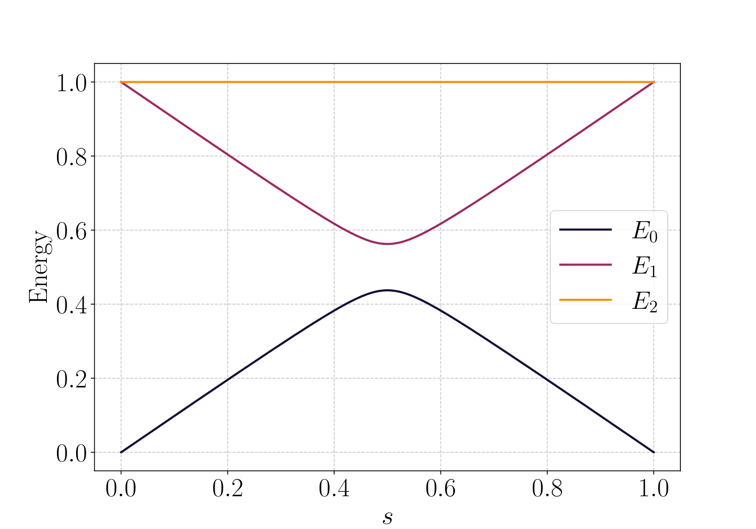
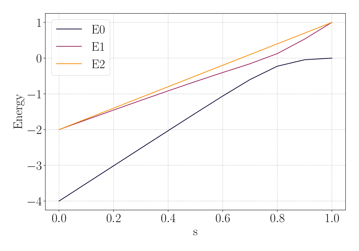
Equation (eqn:Hqaoa): H_Ad(s) = (1-s)H_X + s H_C, with H_X = ∑_i X_i the QAOA mixer chosen as initial Hamiltonian.
Schedule definition (Sec. III-B): the cumulative-integral mapping f(s) with exponent κ=2, normalised so f(0)=0, f(1)=1.
For Grover's problem: g_min is the gap to the first excited state; for MIS it is the gap to the second excited state due to ground-state degeneracy.
Eigenvalue computation: Grover uses a dense scipy.eigh on the n+1-dimensional symmetric subspace; MIS uses sparse scipy.eigsh (Lanczos) for larger sizes.
Extrapolation rule (Sec. IV-D): for n > 12, take the per-s average of the gap profiles from n=6–12, anchored at g(0)=4 and g(1)≈0.
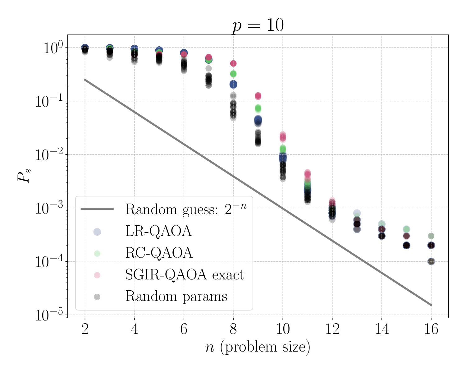
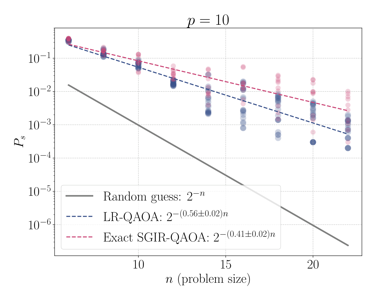
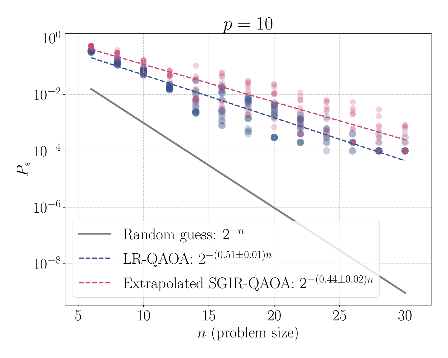
Empirical scaling (Sec. V-B): on degree-3 MIS at p=10, exact SGIR-QAOA gives P_s ∼ 2^{−0.41 n} vs. LR-QAOA's 2^{−0.56 n}; extrapolated SGIR-QAOA still gives 2^{−0.46 n}.

Detailed walkthrough

The paper builds on Linear Ramp QAOA (LR-QAOA, Montanez-Barrera et al. 2025), which fixes β_i = (1 - i/p) Δ_β and γ_i = ((i+1)/p) Δ_γ — a discretised linear adiabatic interpolation. The motivation for SGIR-QAOA is the well-known fact that linear adiabatic schedules destroy Grover's quadratic speed-up: optimal QAA schedules must crawl through the minimum-gap region, satisfying |df/ds| ∝ g(s)², as Roland and Cerf showed in 2002. The novelty here is to compute the gap with respect to H_X (the QAOA mixer) rather than the textbook Grover initial state, on the principle that QAOA is a Trotterised adiabatic algorithm with that specific initial Hamiltonian, so the gap profile in this basis is what governs QAOA's diabatic transitions.

Section III defines the SGIR schedule. The exponent κ=2 is hand-tuned: larger κ concentrates the schedule more sharply around g_min, which the authors find empirically best for the problems studied. The optimisation knobs reduce to two scalars per problem instance — the pre/post-ramp amplitudes — recovering the parameter-economy that motivates LR-QAOA in the first place. A grid search in log-parameter space (logβ ∈ [-1.5, 0.5], logγ ∈ [-1, 1], 11×11) suffices.

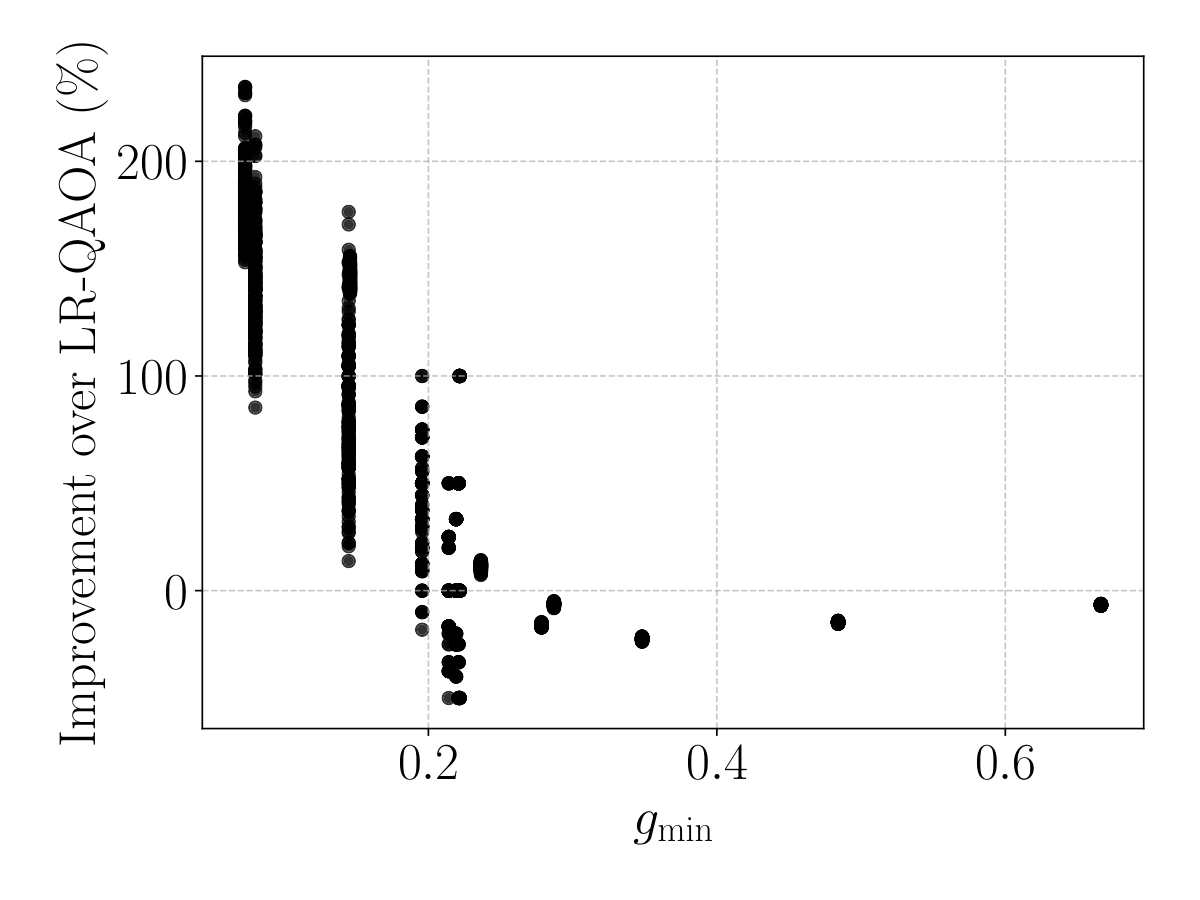
Section V-A validates the method on Grover's search at p=10. The key plot (gap-vs-percent-improvement) shows that SGIR-QAOA's edge over LR-QAOA is most pronounced where g_min is smallest (intermediate n): for n < 6 the gap is large enough that the schedule shape barely matters; for n > 13 at fixed p=10 the discretisation is too coarse to track the adiabatic path in any case. In the productive window 6 ≤ n ≤ 12, SGIR returns the highest P_s. A second plot (depth-to-threshold) shows the depth p required to reach P_s^th=0.1 growing more slowly with n for SGIR-QAOA than for LR-QAOA — a more practically meaningful comparison than constant-p scaling, since on real hardware deeper circuits accumulate more noise.

Section V-B repeats this on degree-3 MIS instances with penalty λ = 2000 chosen deliberately large to push g_min down into the regime where the schedule shape matters. Exact SGIR-QAOA achieves the 2^{−0.41 n} scaling vs. LR-QAOA's 2^{−0.56 n} — a roughly 27% improvement in the exponent. The extrapolated variant uses gaps from n=6–12 to inform schedules for larger n and still produces 2^{−0.46 n}, a meaningful gap to LR-QAOA. This addresses the obvious concern that "schedule needs the gap, but the gap is as hard as the problem" — the gap profile turns out to be smooth and weakly n-dependent, so a small-n template generalises. The same logic applies in Y3's DGMVP context, where the QUBO size could similarly be probed in a small classical regime to inform schedules at scale.

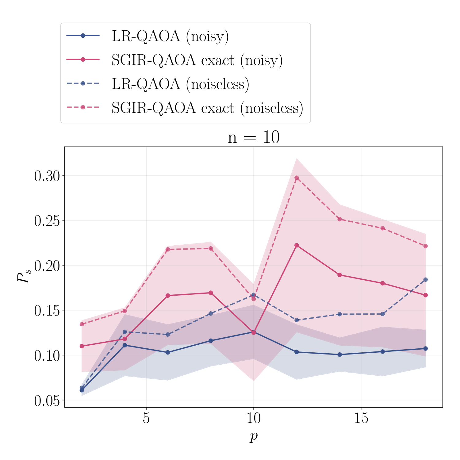
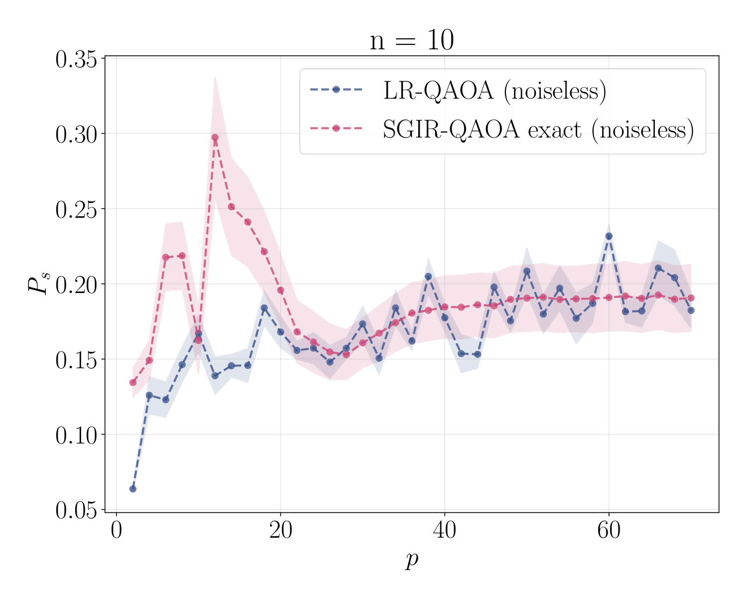
Section V-B-2 (noisy MIS) demonstrates that under depolarising noise p_noise=0.001, SGIR-QAOA's advantage over LR-QAOA persists, and importantly the peak P_s for noisy SGIR-QAOA is reached at smaller p than noiseless LR-QAOA — meaning SGIR effectively buys back some of the depth budget consumed by noise. This is the most operationally interesting result for Yuan's hardware-targeted line of work.

The discussion (Sec. VI) is appropriately cautious: SGIR-QAOA's advantage vanishes in two regimes — (i) when p is so large that even LR-QAOA tracks the adiabatic path, and (ii) when n is so large that even SGIR's slow segments cannot rescue the discretisation. The interesting window is the middle. The authors explicitly flag that follow-up work should compare SGIR-QAOA to classical solvers (cf. weighted Max-Cut benchmarks in Montanez-Barrera et al.) and emphasise the right metric for QAOA runtime is p(n) at threshold probability, not 1/P_s at constant p — a methodological alignment with Y3's runtime analyses.

Figures

Figure 1 (top) — Figure 1 (top half). Eigenvalue spectrum from the conventional Roland-Cerf *H_Ad* for Grover's problem with the marked solution state |000000⟩ (n=6). The minimum gap closes at s=1/2, the canonical adiabatic bottleneck.

Figure 2 (top) — Figure 2 (top half). Eigenvalue spectrum of the SGIR variant *H_Ad(s) = (1-s)H_X + s H_C* for Grover's problem with marked state |0000⟩ (n=4) discretised by p=10. The spectrum has a different shape than the Roland-Cerf version, and the gap minimum sits at s=1.

Figure 3. Solving Grover's problem at constant depth p=10 with LR-QAOA, RC-QAOA, SGIR-QAOA, and QAOA with random parameters. SGIR-QAOA returns the highest *P_s* for 6 < n < 13; beyond n=13 all methods converge as p=10 becomes insufficient.

Figure 4. Correlation between the percent improvement of SGIR-QAOA over LR-QAOA and the minimum spectral gap *g_min*. The advantage grows as *g_min* shrinks — precisely the hard-instance regime where parameter shape matters.

Figure 5. Degree-3 MIS at p=10 and penalty *λ=2000*, exact SGIR-QAOA vs. LR-QAOA. Exponential fits give *2^{−(0.41±0.02) n}* for SGIR vs. *2^{−(0.56±0.02) n}* for LR.

Figure 6. Degree-3 MIS solved at larger n using extrapolated SGIR-QAOA — gaps for n=6–12 inform the schedule for n > 12. The advantage persists.

Figure 7. n=10 MIS instances under depolarising noise *p_noise=0.001*, *λ=100*. Noisy SGIR-QAOA's peak *P_s* sits higher and at lower depth than noisy LR-QAOA, showing the schedule survives mild noise.

Figure 8. Same setup at large p in the noiseless limit, showing convergence of LR and SGIR when p is generous — the SGIR advantage is most useful in the low-budget regime.

Citations to Yuan's papers

No direct citation to any of Y1–Y6 found in bibliography.

Overlap with Y1–Y6

Y1 (warm-started QAOA): Both Y1 and SGIR-QAOA are de-variationalisation strategies: Y1 builds a problem-aware initial state; SGIR builds a problem-aware schedule. They are complementary — SGIR's smooth ramp could initialise Y1's iterative warm-start, or Y1's measurement-derived state could replace the |+⟩ initialisation that SGIR currently inherits from QAOA. The 3-regular MaxCut scaling result in Y1 is directly comparable to SGIR's MIS scaling claims and worth a head-to-head benchmark.
Y2 (quasi-binary portfolio QAOA): Y2's hard mixers preserve the cardinality constraint by construction, while SGIR-QAOA enforces MIS feasibility via a soft penalty λ=2000. SGIR's schedule recipe should transfer to Y2's hard-mixer setup (the gap of (1-s)H_mix^QB + s H_C is the relevant object), and the combination would test whether feasibility-preserving plus gap-informed schedules compound.
Y3 (QAOA DGMVP portfolio): Y3 found that dual annealing + layerwise optimisation was the most robust optimiser. SGIR-QAOA arguably subsumes layerwise: the schedule is fixed by the gap profile, and only two amplitudes need tuning. A direct re-run of Y3's DGMVP benchmarks with SGIR scheduling against Y3's dual-annealing/layerwise pipelines would be a clean comparison — same problem, same QUBO encoding, different parameter pipeline.
Y4 (Grover + ADMM): Tangential here — Grover features in the test bed but the algorithm class is variational, not amplitude-amplification.
Y5 (GW + Pauli sparsity): Largely orthogonal — SGIR-QAOA targets QUBO-style instances, Y5 targets SDP relaxations.
Y6 (PBR Heron2): Unrelated.

Recommended action for Yuan

Read deeper and cite in Y1's next iteration and any QAOA scheduling discussions. SGIR-QAOA is a natural baseline alongside LR-QAOA when arguing for warm-started variants.
Implement for direct comparison on the Y3 DGMVP benchmark. The schedule recipe is short (the cumulative-integral formula plus a κ=2 default) and Yuan already has the QUBO Hamiltonian, eigenvalue routines, and the dual-annealing/layerwise optimisers in place. Reporting SGIR scaling on DGMVP would either strengthen or weaken Y3's pessimism about thermal-noise crossovers.
Email Wallden's group (Edinburgh) or McDowall (NQCC) if Yuan plans to combine SGIR with Y1's warm-start — both teams sit in the same UK quantum-software corridor and a joint angle (warm start × gap-informed schedule) is the kind of integration neither group has yet published.